
EOF Analysis in IDL
QUESTION: Someone told me I should analyze my data in IDL using Principal Component (PC) analysis. Someone else said, no, use Empirical Orthogonal Function (EOF) analysis. I don't know anything about either one of them. Can you help?
![]()
ANSWER: Well, I can try to help, but I strongly recommend you get a copy of Statistical Methods in the Atmospheric Sciences, Second Edition, by Daniel S. Wilks. It may be the most practical statistical book I've ever read. I couldn't do my work without it.
First of all, PC analysis and EOF analysis are one and the same. Edward Lorenz, a Boulder resident who died recently, coined the name Empirical Orthogonal Function analysis when he developed this multivariate statistical technique in the 1950s. (This is the same Lorenz who deeply investigated chaos theory and is famous for illuminating the “butterfly effect.” The text of a talk he gave on the subject, “Predictability: Does the Flap of a Butterfly's Wings in Brazil Set off a Tornado in Texas?” is available for your reading pleasure.) The purpose of EOF analysis is to “reduce a data set containing a large number of variables to a data set containing fewer (hopefully many fewer) new variables.”
In practical terms, we often want to investigate the variability of something like temperature in the Arctic over time. We typically have many thousands of measurements, k, over some finite time, n, and k is much greater than n. In EOF analysis, we are trying to reduce the many-dimensional problem vector space to a reduced set of orthogonal vectors that can be said to “explain ”the variance in the data. It is not unusual in atmospheric science data, which is often highly correlated (temperatures in regions of the Earth near each other do not vary greatly from one another), to find that a handful of vectors, typically five or six of what we call modes, can explain more than 95% of the data variability. Of course, just because we can “explain” the data mathematically doesn't mean that we can explain the underlying physical processes that create the variability in the first place, but that's a science problem, not a programming problem, and I leave that part to you. Many papers, some of them convincing, are written on this topic.
![]()
Obtaining the Data to Analyze
To give us something practical to work on, I have decided to analyze NCEP/NCAR temperature data over the Arctic for the month of September. (Ice concentration minimums are in September, so the idea is that we might understand more about why the Arctic ice is melting if we can see patterns in Arctic temperature variability.) We will begin our analysis in 1987 when ice concentration measurements from satellites became reliable.
The NCEP/NCAR reanalysis data is readily available. The monthly air temperature data set I am interested in is named air.mon.mean.nc and is stored in a netCDF format. The data contains monthly mean temperatures for the years 1969 to present, at 17 different pressure levels (I will be using the 925 mbar pressure in this example). The data is gridded on a global 2.5 degree latitude/longitude grid (144x73). Longitudes range from 0 to 357.5 degrees and latitudes range from -90 to 90 degrees. The complete data set is 144x73x17x722. The last dimension is the number of months since Jan 1969 in units of hours since 01-01-0001. (Don't ask me.) According to the documentation, the air temperature must be prepared for use by multiplying by 0.01 and adding an offset of 127.65.
Here is the code I used to create the data I am going to use in the analysis. To read the data, I used the NCDF_DATA object from the Coyote Library. Running the code results in a data set, named air_temp, containing air temperatures in a 144x18x21 array. In other words, air temperatures measured at 144 times 18 locations (2592 locations), for 21 years. It also results in corresponding latitude and longitude arrays, named ncep_lat and ncep_lon, but these are only used to plot the data from the analysis, they are not used in the analysis itself.
![]()
EOF Analysis
The first step in the EOF analysis is to multiply the air temperature values by a weighting factor, if this is required. In this case it is, because each grid cell in the data is the same size, but each grid cell on the Earth is a different size, according to its latitude. It is common, then, to multiply the data by a “cosine of latitude” weighting factor. I am actually going to use a square-root function of the cosine of latitude, because I think this is more accurate.
Note that my latitude values go from 47.5 to 90.0 degrees of latitude, in 2.5 degree increments. I am going to subtract 1.25 degrees from each of these latitude values, in order to locate the latitudes in the center of the grid, and to avoid multiplying by zero for all the latitudes at 90 degrees.
    dims = Size(air_temp, /Dimensions)
   nlon = dims[0] & nlat = dims[1] & ntime = dims[2]
   lon = Reform(lon_ncep[*,0]) & dlon = Abs(lon[1]-lon[0])
   lat = Reform(lat_ncep[0,*]) & dlat = Abs(lat[1]-lat[0])
   weights = Sqrt(Cos((lat_ncep - dlat/2.) * !DtoR))
   FOR j=0,ntime-1 DO air_temp[*,*,j] = air_temp[*,*,j] * weights
The next step is to reorganize the data into a two-dimensional array of spatial measurements verses time (k verses n, with k >> n). This is easily done in IDL, and results in a 2592 by 21 array.
air_temp = Reform(air_temp, nlon*nlat, ntime, /OVERWRITE)
Normally, the means are subtracted from each spatial point, over time. That is, for each point in space, we calculate the mean value of the 21 time measurements for that point, and subtract that mean from each spatial value. This gives us the data anomalies, or differences. Sometimes the anomalies are divided by the standard deviation of each measurement as well, but since I am going to be doing a covariance analysis, rather than a correlation analysis, this is not necessary here.
    air_anomalies = air_temp
   FOR j=0,nlon*nlat-1 DO air_anomalies[j,*] = air_temp[j,*] - Mean(air_temp[j,*])
Creating the Covariance Matrix: A Trick for Fast Analysis
Since we are concerned with spatial patterns of variance in this analysis, we wish to find out how the spatial patterns vary over time. Thus, the covariance matrix that you would normally want to build would be a 2592x2592 matrix. This is extremely large and difficult to deal with on many computers. If I perform this analysis on a 32-bit computer with 2 GBytes of RAM, the analysis will typically take something in the neighborhood of 25 minutes to run. Running with the complete NCEP temperature array could take hours or days to run.
However, Wilks points out, on page 499 of Statistical Methods, that since k is greater than n, the covariance matrix is singular, which implies that all the eigenvalues after the nth eigenvalue will be approximately zero. Given this, it is pretty much pointless to calculate these additional eigenvalues and their associated eigenvectors, since in practical applications, they will be ignored anyway.
He goes on to point out that rather than creating a k-by-k covariance matrix, the spatial eigenvectors (in other words, the spatial patterns we are looking for) can be recreated by using an n-by-n covariance matrix and reconstructing the n spatial eigenvectors from the n time domain eigenvectors produced by the smaller matrix. This is because the n eigenvalues produced from using the smaller matrix are identical to the n non-zero eigenvalues produced from using the larger matrix. An analysis using this computational trick produces the same results and runs in less than half a second!
Naturally, we are going to use this trick, since you can't believe how much it speeds up program development and debugging! The covariance matrix is calculated like this.
matrix = (1/ntime-1) * (Double(air_anomalies) ## Transpose(air_anomalies))
Just a couple of important points about this. I've tried using the Correlate function to build the correlation matrix, and I find this gives me inaccurate results. My advice to you is to always build the correlation matrix yourself, using code similar to the code above. Note, too, that you must divide the matrix by 1 less than the number of time points you have in the analysis. And keep in mind that the ## operator in IDL multiplies the rows of the first argument by the columns of the second argument, which is what the normal matrix multiplication operator does in linear algebra. You should always use the ## operator, rather than the # operator in these kinds of equations if you wish to be able to read the damn text book at the same time you are coding in IDL. (It seems to me half my time is spent just trying to wrap my head around the differences in (row,col) matrices in the book and IDL's (col,row) arrays in my code! Understanding exactly what the ## operator does helps a lot.)
Calculating the Eigenvectors and Eigenvalues
The next step in the analysis is to calculate the eigenvalues and eigenvectors of the covariance matrix. There are a number of ways to do this in IDL. In this example, I am going to use LA_SVD which uses the mathematical technique called singular value decomposition. This technique will decompose the covariance matrix into a left-matrix of eigenvectors, and a diagonal matrix of singular values, which are the eigenvalues.
LA_SVD, matrix, W, U, V
The variables W, U, and V are the singular values (as a vector), the left-hand matrix, and the right-hand matrix, respectively. These are all output variables and are returned as a result of the decomposition.
The eigenvectors (of the time domain space) are in the columns of U. These will have to be transformed into the eigenvectors of the spatial domain (in the variable eof, below) by the Wilks trick referred to above. In other words, the n-length time domain eigenvectors are converted into the k-length spatial domain eigenvectors. The code looks like this:
    dims = Size(air_anomalies, /Dimensions)
   eof = FltArr(dims[1], dims[0])    FOR j=0,dims[1]-1 DO BEGIN
      t = Transpose(air_anomalies) ## U[j,*]
      eof[j,*]  = t / SQRT(Total(t^2))    ENDFOR
The eigenvectors simply represent the pattern of variance in the spatial measurements. The units are totally arbitrary. The only important characteristic of the values is whether they are positive or negative. To interpret the patterns, we have to look to what are sometimes called the principal components, which are the anomaly data projected onto, or transformed by, or rotated by, (we hear all three of these terms) the eigenvectors. The principal component attached to the corresponding eigenvector spatial pattern provides the sign and overall amplitude of the pattern as a function of time. To calculate the principal component matrix, we execute these commands. The principle component vectors will be the columns of the pc array, and will be of length n.
    pc = FltArr(dims[1], dims[1])
   FOR j=0,dims[1]-1 DO pc[j,*]  = air_anomalies ## eof[j,*]
We sometimes refer to the columns of the eof and pc arrays as the modes. In other words, the first mode is the first column or spatial pattern in the eof array, combined with the first column or PC in the pc array. The first value in the singular value vector corresponds to the first mode, and, as a percentage of the total values, tells you how much the first mode vector “explains” the data variance. We sometimes compute and display this as a percent variance.
percent_variance = W / Total(W) * 100.0
In our case, the first element of the percent_variance vector is about 26, indicated that the first mode explains or predicts about 26% of the variance in the data. The second mode explains about 15% of the variance, and so forth.
Plotting the EOF Analysis
To see how to plot the results of the EOF analysis, let's consider the first mode. We first obtain the first eigenvector (in the first column of the eof variable) and reform it into its spatial dimensions. A number of programs from the Coyote Library are used in this step (e.g, cgScaleVector, cgColor, cgImage, cgLoadCT, and cgSymcat, among others).
    mode = 1    theEOF = eof[mode-1,*]
   theEOF = Reform(theEOF, nlon, nlat, /OVERWRITE)
Next, we open a window and set up the colors for display.
   cgDisplay, 800, 500, /FREE, TITLE='Analysis of NCEP Sept Temperature at 925 mBars'
   cgLoadCT, 3, NCOLORS=128, CLIP=[55, 255]
   cgLoadCT, 1, NCOLORS=127, CLIP=[55, 255], BOTTOM=128, /REVERSE
   TVLCT, cgColor('white', /TRIPLE), 255
The next step is to create a map projection, here an equal area polar projection, and warp the first mode pattern as an image into the map projection. Note the use of the latitude and longitude arrays in the Map_Patch command. Care is taken to scale the data correctly so that negative values are scaled into negative colors, and positive values are scaled into positive colors. Finally, a color bar is added to the plot to give the user some idea of the color scaling. Remember, the actual values are completely arbitrary.
   cgMAP_SET, /LAMBERT, 90, 0, POSITION=[0.025, 0.0, 0.525, 0.8], $
      LIMIT=[45, -180, 90, 180], /NOERASE, /NOBORDER
   value = Max([Abs(Min(theEOF)), Abs(Max(theEOF))] )
   negvalues = Where(theEOF LT 0.0, COMPLEMENT=posvalues)
   negvector = cgScaleVector(findgen(128), -value, 0)
   posvector = cgScaleVector(findgen(127), 0, value)
   negscaled = Value_Locate(negvector, theEOF[negvalues])
   posscaled = Value_Locate(posvector, theEOF[posvalues])    scaled = theEOF
   scaled[negvalues] = negscaled    scaled[posvalues] = posscaled + 128.0
   warp = Map_Patch(scaled, lon_ncep, lat_ncep, /TRIANGULATE, MISSING=255)
   cgImage, warp, POSITION=[0.025, 0.0, 0.525, 0.8]
   cgMap_Continents, COLOR='charcoal'
   cgLoadCT, 3, NCOLORS=128, CLIP=[55, 255]
   cgLoadCT, 1, NCOLORS=127, CLIP=[55, 255], BOTTOM=128, /REVERSE
   cgColorbar, RANGE=[-value, value], DIVISIONS=2, FORMAT='(F8.2)', $
      POSITION=[0.085, 0.875, 0.425,  0.925], ANNOTATECOLOR='navy', XMINOR=0, $
      TITLE='Mode 1 (Sep)', FONT=0, NCOLORS=255
Next, we plot the Principal Component of mode 1.
    time = 21
   years = Indgen(time) + 1987
   cgPlot, years, pc[mode-1,*], /NoErase, COLOR='navy', /NoDATA, $
      TITLE='PC of Mode ' + Strtrim(mode,2) + ' for Sept', FONT=0, $
      POSITION=[0.65, 0.55, 0.95, 0.85], XTITLE='Years', XSTYLE=1
   cgOPlot, years, pc[mode-1,*], COLOR='indian red', THICK=2
   cgOPlot, years, pc[mode-1,*], COLOR='dodger blue', PSYM=16, SYMSIZE=0.75
   cgOPLOT, [!X.CRange[0], !X.CRange[1]], [0, 0], LINESTYLE=2, COLOR='charcoal'
And, finally, we plot the percent variance.
   cgPlot, Indgen(time)+1, percent_variance, /NoErase, COLOR='navy', /NoDATA, $
      TITLE='Percent Variance', FONT=0, XTITLE='Modes', $
      POSITION=[0.65, 0.15, 0.95, 0.38]
   cgOPlot, Indgen(time)+1, percent_variance, COLOR='indian red', THICK=2
   cgOPlot, Indgen(time)+1, percent_variance, COLOR='dodger blue', PSYM=16, SYMSIZE=0.75
   cgPlotS, (Indgen(time)+1)[mode-1], percent_variance[mode-1], COLOR='orange', $
      PSYM=16, SYMSIZE=1.25
You can see the results in the figure below. Here is the code I used to run the program.
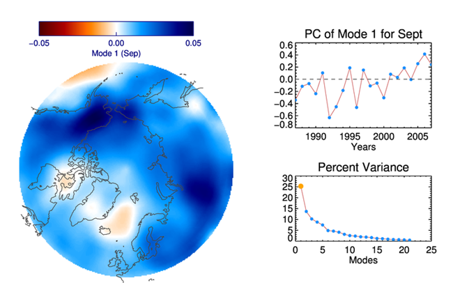 |
| The EOF pattern of the first mode shown on a map projection on the left, and the Principle Component and Percent Varience of the first mode shown on the right. |
![]()
Acknowledgement
My deep appreciation to James McCreight and Mary Jo Brodzik of the National Snow and Ice Data Center and to Balaji Rajagopalan of the University of Colorado for their help in understanding the details of EOF Analysis. Thanks, too, to Tao Wang, who provided me with robust code to use as an example program.
Version of IDL used to prepare this article: IDL 7.0.1.
![]()
Copyright © 2008 David W. Fanning
Last Updated 31 October 2013