
Partioning Values In an Array for Display
QUESTION: I have a 2D array with values ranging from 0.0 to 1.0. I would like to partition the values in this array into a discrete number of colors for display as shown below. What is the best way to do this?
    < 0.2     = White
   0.2 - 0.3 = Green     0.3 - 0.5 = Yellow    0.5 - 0.8 = Blue
   > 0.8     = Red
![]()
ANSWER: The traditional way to do this is to use the Where function to partition the array into these five colors or bins. (Note that if your bin size is constant, which is not the case in this example, the Histogram command is much faster than the Where function for partitioning data into bins.) To see how this works, let's prepare some data for display. As usual, you will need to install the Coyote Library programs in order to run the code below.
data = cgDemoData(11) array = cgScaleVector(data, 0.0, 1.0)
The partitioning is straightforward, if a little tedious to type.
   s = Size(array, /DIMENSIONS)    scaledData = BytArr(s[0], s[1])
   indices = Where(array LT 0.2, count)
   IF count GT 0 THEN scaledData[indices] = 1
   indices = Where(array GE 0.2 AND array LT 0.3, count)
   IF count GT 0 THEN scaledData[indices] = 2
   indices = Where(array GE 0.3 AND array LT 0.5, count)
   IF count GT 0 THEN scaledData[indices] = 3
   indices = Where(array GE 0.5 AND array LT 0.8, count)
   IF count GT 0 THEN scaledData[indices] = 4
   indices = Where(array GT 0.8, count)
   IF count GT 0 THEN scaledData[indices] = 5
To display both the original data and the partitioned array, side by side, you could do something like this.
    !P.Multi = [0,2,1]
   cgdisplay, 600, 300, TITLE='Partitioned Data'    cgLoadCT, 0
   cgImage, data, /KEEP_ASPECT
   TVLCT, cgColor(['white','green','yellow','blue','red'], /TRIPLE), 1
   cgImage, scaledData, /KEEP_ASPECT    !P.Multi = 0
You can see the results in the figure below.
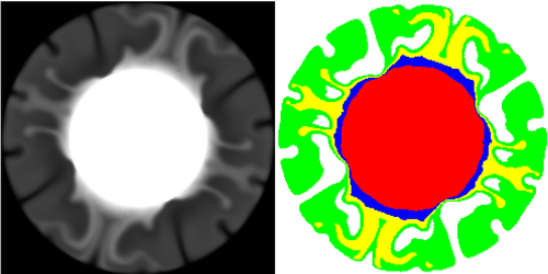 |
| The original data is partitioned into five colors for display. |
![]()
Partitioning the IDL Way
Jeremy Bailin points out that this code can be hard to maintain if you wish to change any of the partitioning values. He suggests an alternative method that takes advantage of Value_Locate to do the partitioning for you. (Value_Locate is becoming one my favorite IDL routines, creeping up on the Where and Histogram functions for its overall usefulness.) I'm pretty jaded when it comes to IDL, but I have to admit, my eyebrows raised when I saw how simply and quickly this works. His way of solving this problem is simply this.
    cutoffs = [0.2, 0.3, 0.5, 0.8]
    scaledData = Byte(Value_Locate(cutoffs, array) + 2)
As you can see from the figure below, the Value_Locate method produces identical results.
   cgDisplay, 400, 450, TITLE='Data Partitioned by VALUE_LOCATE'
  TVLCT, cgColor(['white','green','yellow','blue','red'], /TRIPLE), 1
  cgImage, scaledData, /KEEP_ASPECT, POSITION=[0.1, 0.1, 0.9, 0.8], $
      BACKGROUND='linen'
  cgDCBar, ['white','green','yellow','blue','red'], CHARSIZE=0.75, $
      LABELS=['< 0.2', '0.2-0.3', '0.3-0.5', '0.5-0.8', '> 0.8']
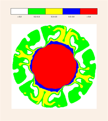 |
| The original data is partitioned into five colors for display. |
![]()
Version of IDL used to prepare this article: IDL 7.0.3.
![]()
Copyright © 2009 David W. Fanning
Last Updated 5 July 2009