Gridding Map Data

QUESTION: I've long thought of GridData as a powerful IDL command that could keep company with Histogram and Value_Locate as valuable and useful commands to know, if I could just get it to work. But, alas, in the many times I've tried to use it, I have never gotten it to work at all. I thought it might do me some good to come clean about my abysmal failure and ask the general public for help. Clearly, there is something simple here I do not understand that goes well beyond foggy documentation. Please contact me with your thoughts and suggestions if you think you might be able to help me see the big picture that I am sure is just out of my visual range.

ANSWER: I have the perfect problem for GridData to attack. I have NCEP temperature anomaly data on a 2.5 degree equirectangular map projection, with associated latitude and longitude variables. The anomaly data is a 144 by 73 floating point array, and the latitude and longitude vectors can be re-created in IDL like this.

    IDL> lat = cgScaleVector(Findgen(73)*2.5), -90, 90)
   IDL> lon = cgScaleVector(Findgen(144)*2.5, 0, 357.5) 

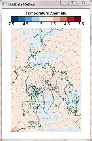
You see what the NCEP data looks like in the figure below. (I have made the tempAnomaly, data available as a binary file if you are interested in trying the code below. It is an array of size (144,73) floating point values.)

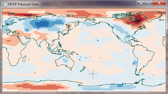The NCEP temperature anomaly data set I wish to grid.

 

I wish to grid this data into a standard polar stereographic grid used at the National Snow and Ice Data Center (NSIDC). You can see details of the grid in the figure below.

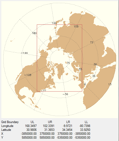The NSIDC Polar Stereographic grid I wish to grid the NCEP data into.

 

This polar stereographic grid is a 304 by 448 grid, with a grid spacing of 25 km. On the figure, you can see the locations of the corners of the grid (the red box) in both latitude and longitude and in X and Y projected grid space.

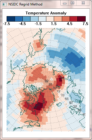
As it happens, I know how to do this kind of regridding in two different ways. First, I can use the regrid command, which is included in a suite of commands for UNIX platforms, named mapx, that NSIDC distributes on their web pages to produce a regridded image I can display. Second, I can use the IDL Contour command, with appropriate projected X and Y location data to produce the same result. You can see the results of these two different methods in the figure below.

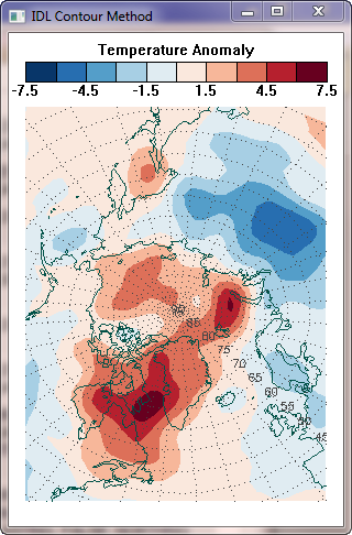Two different methods of gridding the data produce identical results.

 

I am confident these two different methods work and produce the correct results, so this seemed to me to be the perfect opportunity to learn how to do this kind of regridding or interpolation with the GridData command in IDL. The procedure seems absolutely straightforward to me. Use the latitude and longitude vectors (described above) that come with the NCEP temperature anomaly data to produce a projected XY grid. Then regrid this projected data to the NSIDC polar projection, which is described by a second XY grid. It seems to me this is exactly the purpose of the GridData command in IDL. I expected this to be simple to do and I proceeded as follows.

First, read the data. Be sure you reverse the data in the Y direction, since we will be working with maps and IDL uses a convention that is unknown in the mapping world for locating the (0,0) point.

    filename = 'usegriddata.dat'    tempAnomaly= FltArr(144, 73)
   OpenR, lun, filename, /Get_Lun    ReadU, lun, tempAnomaly    Free_Lun, lun
   data = Reverse(tempAnomaly,2) 

Next, make appropriately sized latitude and longitude arrays that correspond to the dimensions of temperature anomaly data. Using the vectors described above (which I actually read out of the netCDF file, but which are easily created in IDL), I executed these commands.

    lat = cgScaleVector(Findgen(73)*2.5), -90, 90)
    lon = cgScaleVector(Findgen(144)*2.5, 0, 357.5)
    ysize = Size(lat, /DIMENSION)     xsize = Size(lon, /DIMENSION)
    lats = Rebin(Reform(lat, 1, ysize), xsize, ysize)
    lons = Rebin(lon, xsize, ysize) 

Next, I set up an equirectangular map projection structure that I can use to convert the latitude and longitude arrays to projected X and Y grid arrays. The code looks like this.

   mapStruct = Map_Proj_Init('Equirectangular', /GCTP, CENTER_LON=180, SPHERE_RADIUS=6378273.00)
   xy = Map_Proj_Forward(lons, lats, MAP_STRUCTURE=mapStruct)
   x = Reform(xy[0,*], xsize, ysize)    y = Reform(xy[1,*], xsize, ysize) 

I want to do the simplest possible thing, so I am going to regrid using nearest neighbor gridding. This is what I used in the NSIDC regrid method described above, and I expect similar results. To use nearest neighbor gridding with GridData, I must supply a set of Delaunay triangles as an input parameter. I create this set of triangles with the Triangulate command in IDL.

    Triangulate, x ,y, triangles 

I am now ready to use GridData. The DELTA parameter is set to a spacing of 25000 meters. The DIMENSIONS parameter is set the to 304 by 448 grid size of the NSIDC polar stereographic projection, and the START parameter is set the the XY values at the lower-left corner of the grid. Here is my code.

    griddedData = GridData(x, y, tempAnomaly, /NEAREST_NEIGHBOR, TRIANGLES=triangles, $
        DELTA=[25000, 25000], DIMENSION=[304,448], START=[-3850000., -5350000.], $
        MISSING=!Values.F_NAN) 

The first thing I noticed is that my data values seem incorrect. The orginal data had values from -5.80780 to 7.08118. The regridded array from the NSIDC regrid command also had these same minimum and maximum values. In the displays above I either scaled the data with this command:

    scaledImage = BytScl(regriddedImage, TOP=9, MIN=-7.5, MAX=7.5) + 1B 

Or, I contoured the data with these levels:

   levels = cgScaleVector(Findgen(10), -7.5, 7.5) 

The griddedData variable from GridData had a minimum value of -0.87048 and a maximum value of 3.28908. If I display it with the same scaling as before, I get the result shown in the figure below, in the middle of my other results.

The GridData method doesn't come close to reproducing the results of the other two methods.

 

But even worse than the data scaling problem, the resulting image doesn't look anything like the results of the other two methods! I'd be greatful for anyone who could take me by the hand and lead me to the promised land.

The Solution

A big "thank-you" to Klemen Zaksek for providing the solution to this problem. It turns out that I needed to turn the latitude and longitude vectors in the input array into the XY locations of the output grid (i.e., the polar stereorgraphic grid). I had actually tried this in my initial attempts to solve this problem, but could not produce the needed set of triangles with the resulting XY arrays. Triangulate kept reporting that the points were "co-linear" and would not produce triangles for me. Of course, these are absolutely required in GridData. So, I thought to try creating triangles with the XY values of the equirectangular grid (as I did above). When this method "worked" (in other words, when I didn't get any errors from Triangulate) I came to the erroneous conclusion that this was the right way to proceed.

I should have done this.

   mapStruct = Map_Proj_Init('Polar Stereographic', /GCTP, CENTER_LON=-45, $
      CENTER_LAT=70, SPHERE_RADIUS=6378273.00)
   xy = Map_Proj_Forward(lons, lats, MAP_STRUCTURE=mapStruct)
   x = Reform(xy[0,*], xsize, ysize)    y = Reform(xy[1,*], xsize, ysize) 

Then, I would have been creating triangles from the right values. But the following Triangulate command would fail on my Windows 64-bit machine, complaining that the input points are co-linear. Strangely, I do not get this error message if I issue the very same command on my 32-bit LINUX machine.

    Triangulate, x ,y, triangles 

To "fix" the problem, I can increase (decrease?) the tolerance that Triangulate has for co-linear points. The following command works on both my LINUX and Windows machines.

    Triangulate, x ,y, triangles, TOLERANCE=1.0 

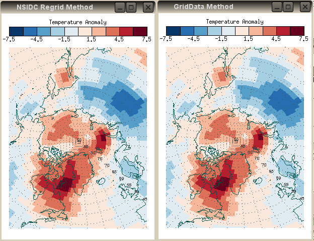
So here is the final result of the GridData method, next to the result of the NSIDC Regrid method. As expected, they are virtually identical.

Used correctly, the IDL GridData method is equivalent to the NSIDC regrid method.

 

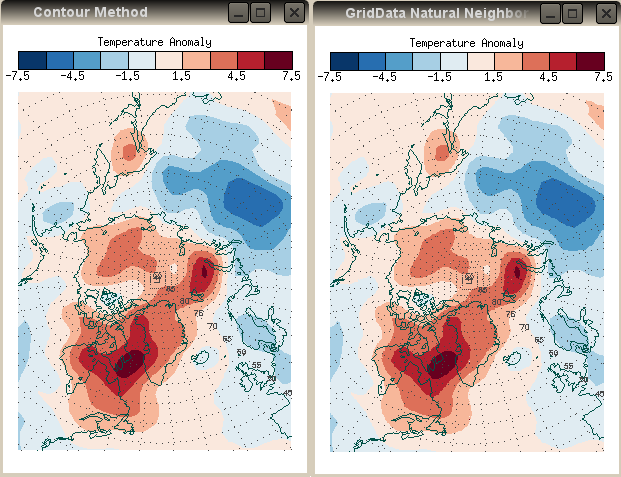
Interestingly, the GridData method, using Natural Neighbor gridding, rather than Nearest Neighbor gridding, is virually identical to the IDL Contour method. If I use the GridData command below, I produce the results shown with the Contour method plot in the figure below.

    griddedData = GridData(x, y, tempAnomaly, /NATURAL_NEIGHBOR, TRIANGLES=triangles, $
        DELTA=[25000, 25000], DIMENSION=[304,448], START=[-3850000., -5350000.], $
        MISSING=!Values.F_NAN) 

The IDL GridData Natural Neighbor method produces results that are indistinguishable from the IDL Contour method results.

 

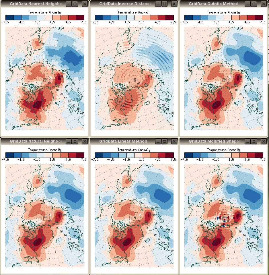
Here is a sample of the various GridData methods, using the same default inputs described above and simply changing the gridding method.

Results from different GridData methods. Left to right, from the top: Nearest Neighbor, Inverse Distance (the default method), Quintic, Natural Neighbor, Linear Interpolation, Modified Shepard's Interpolation.

 

The figures above were created on my 32-bit UNIX machine. If I run the very same code on my Windows machine (64-bit, Windows 7 OS), the Modified Shepard's Interpolation method looks quite different, as shown below. I do not have an explanation for why GridData gives different results on different machines.

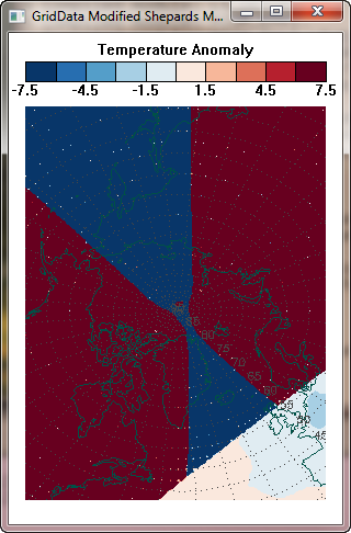The Modified Shepard's Interpolation method produces quite different results on a 64-bit Windows 7 machine compared to a 32-bit LINUX machine.

 

Faster Gridding

If you have a regular data grid, as here. And you just want to organize the data into another regular grid, as here, and you can live with nearest neightbor, bilinear, or cubic interpolation, then it is much, much faster to use the Interpolate function rather than GridData to do the gridding. While this is orders of magnitude faster, I have always found it harder to get my head around how to do it. In particular, I have found it especially difficult to understand how to obtain the fractional index values I need for the interpolation. The method I outline here is beginning to make some sense to me!

As before, let's read the data. Notice that we reverse the data in the Y direction. This is just standard procedure when working with data and maps in IDL, and is used to align IDL's notion of the (0,0) point in the array to the mapping world's notion of its location. We also store the dimensions of the data array, as we will need this later.

   filename = 'usegriddata.dat'    tempAnomaly= FltArr(144, 73)
   OpenR, lun, filename, /Get_Lun    ReadU, lun, tempAnomaly    Free_Lun, lun
   tempAnomaly = Reverse(tempAnomaly, 2)
   dims = Size(tempAnomaly, /DIMENSIONS) 

Next, we set up map projection and grids that describe the study space. In versions of IDL prior to IDL 8, a Polar Stereographic projection had to be set up using the wrong keywords.

     IF Float(!Version.Release) GE 8.0 THEN BEGIN
       map = Obj_New('cgMap', 'Polar Stereographic', /GCTP, CENTER_LON=-45, $
         TRUE_SCALE_LATITUDE=70, SPHERE_RADIUS=6378273.00)     ENDIF ELSE BEGIN
       map = Obj_New('cgMap', 'Polar Stereographic', /GCTP, CENTER_LON=-45, $
         CENTER_LAT=70, SPHERE_RADIUS=6378273.00)     ENDELSE
   x0 = -3850000.0D    x1 = 3750000.0D    y0 = -5350000.0D    y1 = 5850000.0D
   xdim = 304    ydim = 448    xscale = (x1 - x0) / xdim
   yscale = (y1 - y0) / ydim
   xvec = cgScaleVector(Findgen(xdim), x0+(xscale/2.0), x1-(xscale/2.0))
   yvec = cgScaleVector(Findgen(ydim), y0+(yscale/2.0), y1-(yscale/2.0))
   xgrid = Rebin(xvec, xdim, ydim)
   ygrid = Rebin(Reform(yvec, 1, ydim), xdim, ydim) 

Next, we turn these XY projected meter grid points into the latitude and longitude values used by the input data.

   latlon = map -> Inverse(xgrid, ygrid)
   longrid = Reform(latlon[0,*], xdim, ydim)
   latgrid = Reform(latlon[1,*], xdim, ydim) 

It is essential, at this point, to make sure our longitude values are in the range of 0 to 360, and not in the range -180 to 180. We force the longitudes into this range with this command.

   longrid = (longrid + 360) MOD 360 

Now, here is the tricky part. We want to turn these new gridded longitude and latitude arrays into fractional indices of the original input data values. We can do this with the Coyote Library routine cgScaleVector. Essentially, we scale the values of the grids into the dimensions of the input data.

    xindex = cgScaleVector(longrid, 0, dims[0], Min=0.0, Max=357.5)
   yindex = cgScaleVector(latgrid, 0, dims[1], Min=-90.0, Max=90.0) 

Finally, we simply use these fractional index arrays to interpolate the the original data. We can use either nearest neighbor, bilinear, or cubic interpolation.

    nearestNeighbor = tempAnomaly[Round(xindex), Round(yindex)]
    bilinear = Interpolate(tempAnomaly, xindex, yindex)
    cubic = Interpolate(tempAnomaly, xindex, yindex, /Cubic) 

We can display the data with code similar to this (I am showing the code for the bilinear gridded data here).

    cgDisplay, 300, 450, /Free, Title='Bilinear Interpolation'
    mapPosition = [0.05, 0.05, 0.95, 0.85]
    map -> SetProperty, XRange=[x0,x1], YRange=[y0,y1], Position=mapPosition
    map -> Draw     cgLoadCT, 22, /Reverse, NColors=10, Bottom=1, /Brewer
    scaledImage = BytScl(nearestNeighbor, TOP=9, MIN=-7.5, MAX=7.5) + 1B
    cgImage, scaledImage, Position=mapPosition
    names = String(Findgen(11)*1.5-7.5, Format='(F0.1)')
    names[indgen(5)*2+1] = " "
    cgColorbar, NColors=10, Bottom=1, /Discrete, Range=[-7.5, 7.5], $
       Ticknames=names, Position=[0.05, 0.9, 0.95, 0.93], Title='Temperature Anomaly', $
       Charsize=0.75
    Map_Grid, MAP=map->GetMapStruct(), Lats=Indgen(10)*10, Lons=Indgen(36)*10, Color=cgColor('black')
    cgMap_Continents, Map=map 

You see the results of the gridding in the figure below.

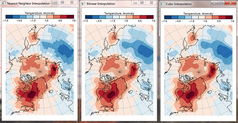With regular arrays, the gridding can be accomplished orders of magnitude faster with interpolation.

 

A program, named FastGridding, is available to run the code above.

For additional information on this topic, please see the article Gridding Irregular Data.

Version of IDL used to prepare this article: IDL 7.1.2