| cgGallery with function graphics [message #87787] |
Thu, 27 February 2014 06:46  |
 Matthew Argall
Messages: 286
Registered: October 2011
|
Senior Member |
|
|
Hi, all,
I thought I would create a thread with examples from the coyote gallery reproduced with function graphics. It is sort of my learning process. I will also include comments regarding some of the non-intuitiveness / problems (bugs?) that I am running into as I try to use function graphics more.
I will post each reproduction as a reply to this, and will dredge up the thread in the future when if I get around to creating more. Feel free to do the same. Also, comments and fixes are welcome.
http://www.idlcoyote.com/gallery/
For good measure
IDL> print, !version
{ x86_64 darwin unix Mac OS X 8.2 Apr 10 2012 64 64}
|
|
|
|
| Re: cgGallery with function graphics [message #87788 is a reply to message #87787] |
Thu, 27 February 2014 06:46  |
Matthew Argall
Messages: 286
Registered: October 2011
|
Senior Member |
|
|
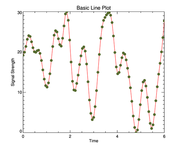
Basic Line Plot
http://www.idlcoyote.com/gallery/basic_line_plot.png
; Example data.
data = cgDemoData(1)
time = cgScaleVector(Findgen(N_Elements(data)), 0, 6)
; Set up variables for the plot. Normally, these values would be
; passed into the program as positional and keyword parameters.
xtitle = 'Time'
ytitle = 'Signal Strength'
title = 'Basic Line Plot'
position = [0.125, 0.125, 0.9, 0.925]
;Create the plot
fgPlot = Plot(time, data, Color='red', Symbol="Circle", Sym_Color='Olive_Drab', /Sym_Filled, $
Sym_Size=1.0, Title=title, XTitle=xtitle, YTitle=ytitle, $
Position=position)
|
|
|
|
| Re: cgGallery with function graphics [message #87789 is a reply to message #87787] |
Thu, 27 February 2014 06:48 |
Matthew Argall
Messages: 286
Registered: October 2011
|
Senior Member |
|
|
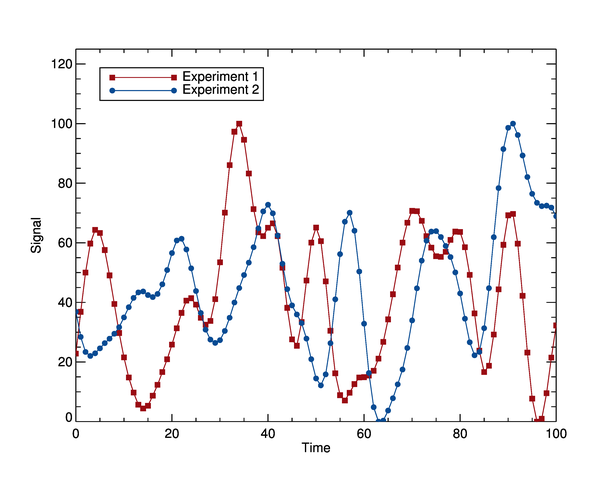
Line Plot With Legend
http://www.idlcoyote.com/gallery/plot_with_legend.png
; Set up variables for the plot. Normally, these values would be
; passed into the program as positional and keyword parameters.
; Create two random vectors.
data_1 = cgDemoData(17)
data_2 = cgDemoData(17)
; Calculate the data range, so you can create a plot with room at the top
; of the plot for the legend.
maxData = Max(data_1) > Max(data_2)
minData = Min(data_1) > Min(data_2)
dataRange = maxData - minData
yrange = [MinData, maxData + (dataRange*0.25)]
; Legend Properties
items = ['Experiment 1', 'Experiment 2']
psyms = [-15, -16]
colors = ['red7', 'blu7']
;Plot the data
ngPlot = Plot(data_1, Symbol='Circle', /Sym_Filled, Color='Red', YRange=yrange, YStyle=1, $
XTitle='Time', YTitle='Signal', Name='Experiment 1')
ngOPlot = Plot(data_2, Symbol='Square', /Sym_Filled, Color='Blue', Overplot=ngPlot, $
Name='Experiment 2')
|
|
|
|
| Re: cgGallery with function graphics [message #87790 is a reply to message #87787] |
Thu, 27 February 2014 06:56 |
Matthew Argall
Messages: 286
Registered: October 2011
|
Senior Member |
|
|
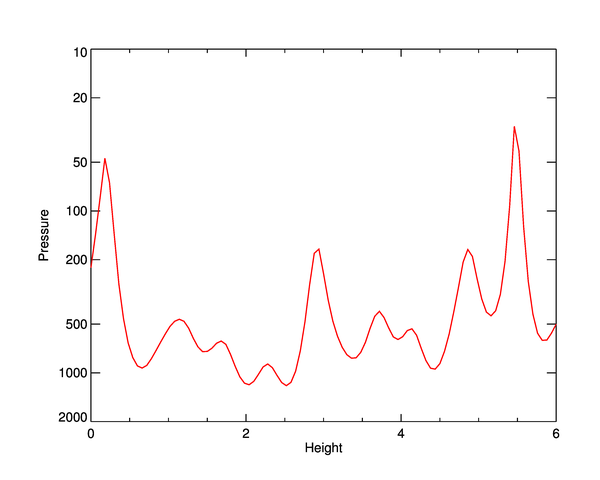
Logarithmic Pressure Plot
http://www.idlcoyote.com/gallery/logarithmic_pressure_plot.p ng
; Example data. Normally passed into the program as a positional parameter.
data = cgScaleVector(cgDemoData(1), 30, 1200)
height = cgScaleVector(Findgen(N_Elements(data)), 0, 6)
thick = 2
; To label minor ticks on the axis use Martin Shultz program LogLevels.
; Set YTICKS to one less than the number of ticks returned by LogLevels.
ticks = LogLevels([10,2000])
nticks = N_Elements(ticks)
; Draw a plot with the Y axis labelled as a reversed logarithmic axis.
ngPlot = Plot(height, data, /YLOG, YRANGE=[2000,10], $
XTitle='Height', YTitle='Pressure', Color='Red')
(ngPlot.Axes)[1].tickvalues = ticks
|
|
|
|
| Re: cgGallery with function graphics [message #87791 is a reply to message #87787] |
Thu, 27 February 2014 07:01 |
David Fanning
Messages: 11724
Registered: August 2001
|
Senior Member |
|
|
Matthew Argall writes:
>
> Hi, all,
>
> I thought I would create a thread with examples from the coyote gallery reproduced with function graphics. It is sort of my learning process. I will also include comments regarding some of the non-intuitiveness / problems (bugs?) that I am running into as I try to use function graphics more.
>
> I will post each reproduction as a reply to this, and will dredge up the thread in the future when if I get around to creating more. Feel free to do the same. Also, comments and fixes are welcome.
>
> http://www.idlcoyote.com/gallery/
>
>
> For good measure
> IDL> print, !version
> { x86_64 darwin unix Mac OS X 8.2 Apr 10 2012 64 64}
Hi Matt,
This has been on my to-do list for awhile now, too. I'm happy to publish
these for you as additional information in the Gallery. It would be
helpful if we could keep the same format for the code. It would be
useful if the code also produces a PostScript and PNG file of the plot.
This make it easier to add to my web page and it allows people to
directly compare results.
Cheers,
David
--
David Fanning, Ph.D.
Fanning Software Consulting, Inc.
Coyote's Guide to IDL Programming: http://www.idlcoyote.com/
Sepore ma de ni thue. ("Perhaps thou speakest truth.")
|
|
|
|
|
|
| Re: cgGallery with function graphics [message #87793 is a reply to message #87789] |
Thu, 27 February 2014 07:32 |
Paul Van Delst[1]
Messages: 1157
Registered: April 2002
|
Senior Member |
|
|
You forgot the call to LEGEND().
On 02/27/14 09:48, Matthew Argall wrote:
> Line Plot With Legend
> http://www.idlcoyote.com/gallery/plot_with_legend.png
>
> ; Set up variables for the plot. Normally, these values would be
> ; passed into the program as positional and keyword parameters.
> ; Create two random vectors.
> data_1 = cgDemoData(17)
> data_2 = cgDemoData(17)
>
> ; Calculate the data range, so you can create a plot with room at the top
> ; of the plot for the legend.
> maxData = Max(data_1) > Max(data_2)
> minData = Min(data_1) > Min(data_2)
> dataRange = maxData - minData
> yrange = [MinData, maxData + (dataRange*0.25)]
>
> ; Legend Properties
> items = ['Experiment 1', 'Experiment 2']
> psyms = [-15, -16]
> colors = ['red7', 'blu7']
>
> ;Plot the data
> ngPlot = Plot(data_1, Symbol='Circle', /Sym_Filled, Color='Red', YRange=yrange, YStyle=1, $
> XTitle='Time', YTitle='Signal', Name='Experiment 1')
> ngOPlot = Plot(data_2, Symbol='Square', /Sym_Filled, Color='Blue', Overplot=ngPlot, $
> Name='Experiment 2')
>
|
|
|
|
| Re: cgGallery with function graphics [message #87794 is a reply to message #87790] |
Thu, 27 February 2014 07:35 |
David Fanning
Messages: 11724
Registered: August 2001
|
Senior Member |
|
|
Matthew Argall writes:
>
> Logarithmic Pressure Plot
> http://www.idlcoyote.com/gallery/logarithmic_pressure_plot.p ng
>
>
> ; Example data. Normally passed into the program as a positional parameter.
> data = cgScaleVector(cgDemoData(1), 30, 1200)
> height = cgScaleVector(Findgen(N_Elements(data)), 0, 6)
> thick = 2
>
> ; To label minor ticks on the axis use Martin Shultz program LogLevels.
> ; Set YTICKS to one less than the number of ticks returned by LogLevels.
> ticks = LogLevels([10,2000])
> nticks = N_Elements(ticks)
>
> ; Draw a plot with the Y axis labelled as a reversed logarithmic axis.
> ngPlot = Plot(height, data, /YLOG, YRANGE=[2000,10], $
> XTitle='Height', YTitle='Pressure', Color='Red')
> (ngPlot.Axes)[1].tickvalues = ticks
Unfortunately, this plot doesn't work in my version of IDL (8.2.3). I
get two X axes with the text all jumbled together in one place. I'll be
sending all inquires about this to your e-mail. ;-)
Cheers,
David
--
David Fanning, Ph.D.
Fanning Software Consulting, Inc.
Coyote's Guide to IDL Programming: http://www.idlcoyote.com/
Sepore ma de ni thue. ("Perhaps thou speakest truth.")
|
|
|
|
| Re: cgGallery with function graphics [message #87795 is a reply to message #87787] |
Thu, 27 February 2014 07:35 |
Matthew Argall
Messages: 286
Registered: October 2011
|
Senior Member |
|
|
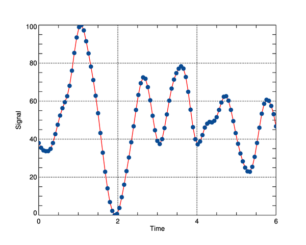
Grid On Line Plot
http://www.idlcoyote.com/gallery/grid_plot.png
==============
Copy + Paste Version
==============
; Example data. Normally passed into the program as a positional parameter.
data = cgScaleVector(cgDemoData(1), 30, 1200)
height = cgScaleVector(Findgen(N_Elements(data)), 0, 6)
thick = 2
; To label minor ticks on the axis use Martin Shultz program LogLevels.
; Set YTICKS to one less than the number of ticks returned by LogLevels.
ticks = LogLevels([10,2000])
nticks = N_Elements(ticks)
; Create the plot
ngPlot = Plot(time, data, Thick=thick, Color='Red', XTitle='Time', $
YTitle='Signal', Symbol='Circle', /Sym_Filled, Sym_Size=1.5, $
Sym_Color='Blue')
; Add the grid
; Note: There is a bug in IDL 8.2 that applies a minor tickmark grid for half of the grid.
(ngPlot.Axes)[0].TickLen = 1
(ngPlot.Axes)[0].GridStyle = 1
(ngPlot.Axes)[1].TickLen = 1
(ngPlot.Axes)[1].GridStyle = 1
============================================
Coyote Version
============================================
PRO Grid_On_Line_Plot_FG, WINDOW=window
; Example data. Normally passed into the program as a positional parameter.
data = cgScaleVector(cgDemoData(1), 30, 1200)
height = cgScaleVector(Findgen(N_Elements(data)), 0, 6)
thick = 2
; To label minor ticks on the axis use Martin Shultz program LogLevels.
; Set YTICKS to one less than the number of ticks returned by LogLevels.
ticks = LogLevels([10,2000])
nticks = N_Elements(ticks)
; Open a window and return its reference to the user.
aWindow = Window(WINDOW_TITLE="Grid on Line Plot")
; Create the plot
ngPlot = Plot(time, data, /Current, Thick=thick, Color='Red', XTitle='Time', $
YTitle='Signal', Symbol='Circle', /Sym_Filled, Sym_Size=1.5, $
Sym_Color='Blue')
; Add the grid
; Note: There is a bug in IDL 8.2 that applies a minor tickmark grid for half of the grid.
(ngPlot.Axes)[0].TickLen = 1
(ngPlot.Axes)[0].GridStyle = 1
(ngPlot.Axes)[1].TickLen = 1
(ngPlot.Axes)[1].GridStyle = 1
END ;*********************************************************** ******
; This main program shows how to call the program and produce
; various types of output.
; Display the plot in a resizeable graphics window.
Grid_On_Line_Plot_FG, Window=window
; Create a PostScript file. Linestyles are not preserved in IDL 8.2.3 due
; to a bug. Only encapsulated PostScript files can be created.
window.save, 'grid_on_line_plot_fg.eps'
; Create a PNG file with a width of 600 pixels. Resolution of this
; PNG file is not very good.
window.save, 'grid_on_line_plot_fg.png', WIDTH=600
; For better resolution PNG files, make the PNG full-size, then resize it
; with ImageMagick. Requires ImageMagick to be installed.
window.save, 'additional_axes_plot_fg_fullsize.png'
Spawn, 'convert grid_on_line_plot_fg_fullsize.png -resize 600 grid_on_line_plot_fg_resized.png'
END
|
|
|
|
|
|
|
|
| Re: cgGallery with function graphics [message #87798 is a reply to message #87787] |
Thu, 27 February 2014 07:45 |
Paul Van Delst[1]
Messages: 1157
Registered: April 2002
|
Senior Member |
|
|
The only comment, well, request, I have is that you post the timing for
the plots also (e.g. using tic/toc).
For the simpler plots/smaller datasets there's probably no difference.
The extreme slowness of function- compared to direct-graphics should
continually be highlighted so that it gets addressed in future IDL releases.
<soapbox mounted=true>
For the record, I use FG pretty much exclusively. I think they're great.
However, when I truly need to inspect a dataset (and I work with
satellite data so the datasets are large by default :o) by plotting it
multiple times quickly in several different ways, zooming, overplotting,
redisplaying, etc I *have* to use direct/coyote graphics.
E.g. Plotting and zooming in/out of multiple fourier interpolated
radiance spectra that each contain 2^18 points is simply not reasonable
in IDL FG. I've been doing that in DG for (gulp) decades.
Other E.g. displaying multiple maps of global satellite data (or its
products) coverage.
Other (unmentioned) products have OOG capabilities that do not suffer
from this speed problem so one can only assume it's an implementation issue.
</soapbox>
cheers,
paulv
On 02/27/14 09:46, Matthew Argall wrote:
> Hi, all,
>
> I thought I would create a thread with examples from the coyote
> gallery reproduced with function graphics. It is sort of my learning
> process. I will also include comments regarding some of the
> non-intuitiveness / problems (bugs?) that I am running into as I try
> to use function graphics more.
>
> I will post each reproduction as a reply to this, and will dredge up
> the thread in the future when if I get around to creating more. Feel
> free to do the same. Also, comments and fixes are welcome.
>
> http://www.idlcoyote.com/gallery/
>
>
> For good measure IDL> print, !version { x86_64 darwin unix Mac OS X
> 8.2 Apr 10 2012 64 64}
>
|
|
|
|
| Re: cgGallery with function graphics [message #87799 is a reply to message #87793] |
Thu, 27 February 2014 07:46 |
Matthew Argall
Messages: 286
Registered: October 2011
|
Senior Member |
|
|
Woops! Here it is in its entirety (with the legend and coyote version)
=================
Copy + Paste
=================
; Set up variables for the plot. Normally, these values would be
; passed into the program as positional and keyword parameters.
; Create two random vectors.
data_1 = cgDemoData(17)
data_2 = cgDemoData(17)
; Calculate the data range, so you can create a plot with room at the top
; of the plot for the legend.
maxData = Max(data_1) > Max(data_2)
minData = Min(data_1) > Min(data_2)
dataRange = maxData - minData
yrange = [MinData, maxData + (dataRange*0.25)]
; Legend Properties
items = ['Experiment 1', 'Experiment 2']
psyms = [-15, -16]
colors = ['red7', 'blu7']
; Open a window and return its reference to the user.
aWindow = Window(WINDOW_TITLE="Line Plot with Legend")
;Create the Plot
ngPlot = Plot(data_1, /Current, Symbol='Circle', /Sym_Filled, Color='Red', $
YRange=yrange, YStyle=1, XTitle='Time', YTitle='Signal', $
Name='Experiment 1')
ngOPlot = Plot(data_2, Symbol='Square', /Sym_Filled, Color='Blue', $
Overplot=ngPlot, Name='Experiment 2')
;Add the legend
ngLegend = Legend(/Auto_Text_Color, Position=[5, 120], Target=[ngPlot, ngOPlot], /Data, $
Horizontal_Alignment='Left')
=================
Coyote Version
=================
PRO Line_Plot_With_Legend_FG, WINDOW=window
; Set up variables for the plot. Normally, these values would be
; passed into the program as positional and keyword parameters.
; Create two random vectors.
data_1 = cgDemoData(17)
data_2 = cgDemoData(17)
; Calculate the data range, so you can create a plot with room at the top
; of the plot for the legend.
maxData = Max(data_1) > Max(data_2)
minData = Min(data_1) > Min(data_2)
dataRange = maxData - minData
yrange = [MinData, maxData + (dataRange*0.25)]
; Legend Properties
items = ['Experiment 1', 'Experiment 2']
psyms = [-15, -16]
colors = ['red7', 'blu7']
; Open a window and return its reference to the user.
aWindow = Window(WINDOW_TITLE="Line Plot with Legend")
;Create the Plot
ngPlot = Plot(data_1, /Current, Symbol='Circle', /Sym_Filled, Color='Red', $
YRange=yrange, YStyle=1, XTitle='Time', YTitle='Signal', $
Name='Experiment 1')
ngOPlot = Plot(data_2, Symbol='Square', /Sym_Filled, Color='Blue', $
Overplot=ngPlot, Name='Experiment 2')
;Add the legend
ngLegend = Legend(/Auto_Text_Color, Position=[5, 120], Target=[ngPlot, ngOPlot], /Data, $
Horizontal_Alignment='Left')
END ;*********************************************************** ******
; This main program shows how to call the program and produce
; various types of output.
; Display the plot in a resizeable graphics window.
Line_Plot_With_Legend_FG, Window=window
; Create a PostScript file. Linestyles are not preserved in IDL 8.2.3 due
; to a bug. Only encapsulated PostScript files can be created.
window.save, 'ling_plot_with_legend.eps'
; Create a PNG file with a width of 600 pixels. Resolution of this
; PNG file is not very good.
window.save, 'ling_plot_with_legend.png', WIDTH=600
; For better resolution PNG files, make the PNG full-size, then resize it
; with ImageMagick. Requires ImageMagick to be installed.
window.save, 'ling_plot_with_legend_fullsize.png'
Spawn, 'convert ling_plot_with_legend_fg_fullsize.png -resize 600 ling_plot_with_legend_fg_resized.png'
END
|
|
|
|
|
|
|
|
| Re: cgGallery with function graphics [message #87802 is a reply to message #87787] |
Thu, 27 February 2014 08:13 |
Matthew Argall
Messages: 286
Registered: October 2011
|
Senior Member |
|
|
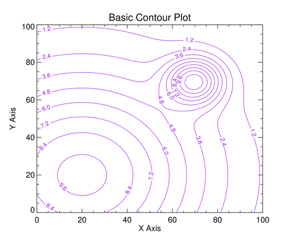
Basic Contour Plot
http://www.idlcoyote.com/gallery/basic_contour_plot.png
=================
Copy + Paste
=================
; Example Gaussian data.
data = cgDemoData(26)
; Set up variables for the contour plot. Normally, these values
; would be passed into the program as positional and keyword parameters.
minValue = Floor(Min(data))
nLevels = 10
xtitle = 'X Axis'
ytitle = 'Y Axis'
position = [0.125, 0.125, 0.9, 0.9]
title = 'Basic Contour Plot'
;Contour levels
contourLevels = cgConLevels(data, NLevels=10, MinValue=minValue)
; Open a window and return its reference to the user.
aWindow = Window(WINDOW_TITLE="Basic Contour Plot")
;Create a contour
fgContour = Contour(data, /Current, C_Value=contourLevels, C_Color='Purple', $
XTitle=xtitle, YTitle=ytitle, Title=title)
;Add the right and top axes
; In IDL 8.2.3+ set Location='Right' or 'Top' and skip finding [xy]range.
xrange = (fgContour.Axes)[0].Range
yrange = (fgContour.Axes)[1].Range
xAxis = Axis('X', Target=fgContour, Location=[xrange[1], yrange[1], 0], $
TickFormat='(A1)', TickDir=1)
yAxis = Axis('Y', Target=fgContour, Location=[xrange[1], yrange[0], 0], $
TickFormat='(A1)', TickDir=1)
=================
Coyote Version
=================
PRO Basic_Contour_Plot_FG, WINDOW=window
; Example Gaussian data.
data = cgDemoData(26)
; Set up variables for the contour plot. Normally, these values
; would be passed into the program as positional and keyword parameters.
minValue = Floor(Min(data))
nLevels = 10
xtitle = 'X Axis'
ytitle = 'Y Axis'
position = [0.125, 0.125, 0.9, 0.9]
title = 'Basic Contour Plot'
;Contour levels
contourLevels = cgConLevels(data, NLevels=10, MinValue=minValue)
; Open a window and return its reference to the user.
aWindow = Window(WINDOW_TITLE="Basic Contour Plot")
;Create a contour
fgContour = Contour(data, /Current, C_Value=contourLevels, C_Color='Purple', $
XTitle=xtitle, YTitle=ytitle, Title=title)
;Add the right and top axes
; In IDL 8.2.3+ set Location='Right' or 'Top' and skip finding [xy]range.
xrange = (fgContour.Axes)[0].Range
yrange = (fgContour.Axes)[1].Range
xAxis = Axis('X', Target=fgContour, Location=[xrange[1], yrange[1], 0], $
TickFormat='(A1)', TickDir=1)
yAxis = Axis('Y', Target=fgContour, Location=[xrange[1], yrange[0], 0], $
TickFormat='(A1)', TickDir=1)
END ;*********************************************************** ******
; This main program shows how to call the program and produce
; various types of output.
; Display the plot in a resizeable graphics window.
Basic_Contour_Plot_FG, Window=window
; Create a PostScript file. Linestyles are not preserved in IDL 8.2.3 due
; to a bug. Only encapsulated PostScript files can be created.
window.save, 'basic_contour_plot_fg.eps'
; Create a PNG file with a width of 600 pixels. Resolution of this
; PNG file is not very good.
window.save, 'basic_contour_plot_fg.png', WIDTH=600
; For better resolution PNG files, make the PNG full-size, then resize it
; with ImageMagick. Requires ImageMagick to be installed.
window.save, 'line_plot_with_legend_fullsize.png'
Spawn, 'convert basic_contour_plot_fg_fullsize.png -resize 600 basic_contour_plot_fg_resized.png'
END
|
|
|
|
| Re: cgGallery with function graphics [message #87803 is a reply to message #87800] |
Thu, 27 February 2014 08:22 |
David Fanning
Messages: 11724
Registered: August 2001
|
Senior Member |
|
|
David Fanning writes:
>
> Paul van Delst writes:
>
>> The only comment, well, request, I have is that you post the timing for
>> the plots also (e.g. using tic/toc).
>
> I don't know. There are a LOT of factors here. I'm not sure the numbers
> will allow us to compare apples with apples. I think we should just
> allow people to time things themselves. Then, the test is strictly based
> on how they are using the routines. Plus, many of the Coyote Graphics
> users don't have Tic and Toc. :-)
Just to give you an example. I ran both the Coyote Graphics and Function
Graphics basic line plot routines first to "initialize" the system.
Then I timed just the time to produce a plot.
Coyote Graphics: 0.0300 ; Probably slow because of circle symbol
Function Graphics: 0.0268
Then I timed the time to produce the plot and make a PostScript and PNG
file:
Coyote Graphics: 1.672
Function Graphics: 4.398 ; Probably slow because of big PNG file
If I make a big PNG file with Coyote Graphics, then I get a time of
3.091.
So, I don't know. My impression is always that Function Graphics
routines are slower, but I have no idea how MUCH slower. I think if you
have a reasonable high tolerance for complicated things not always
working right, you are probably OK with function graphics. In my tests
of hardcopy output (the only thing I really care about, usually), I find
Coyote Graphics work more intuitively than Function Graphics and produce
identical results. When I build applications that are to go in front of
a user, I tend to use object graphics, but only because I find these a
little more reliable than function graphics. (The pressure plot saga of
this morning seems to happen to me a LOT when I use function graphics. I
think I must have an undiscovered and unintentional talent for breaking
those things!)
Cheers,
David
--
David Fanning, Ph.D.
Fanning Software Consulting, Inc.
Coyote's Guide to IDL Programming: http://www.idlcoyote.com/
Sepore ma de ni thue. ("Perhaps thou speakest truth.")
|
|
|
|
|
|
|
|
| Re: cgGallery with function graphics [message #87806 is a reply to message #87804] |
Thu, 27 February 2014 08:51 |
Matthew Argall
Messages: 286
Registered: October 2011
|
Senior Member |
|
|
> Uh, OK. Are you alright with the contour labels being upside down? Is
> that something you might be able to fix?
I tried for quite a while to reverse the labels, but could not figure out how... Unless I specify my own IDLgrSymbol or IDLgrText object through the C_Label_Object.
The colors are purple for me, not orange, and none of them are faint.
I should add that I forgot to include the C_Label_Show keyword to get the labels to appear, so the contour plot should look like this
fgContour = Contour(data, /Current, C_Value=contourLevels, C_Color='Purple', $
XTitle=xtitle, YTitle=ytitle, Title=title, C_Label_Show=1)
|
|
|
|
| Re: cgGallery with function graphics [message #87807 is a reply to message #87806] |
Thu, 27 February 2014 08:55 |
David Fanning
Messages: 11724
Registered: August 2001
|
Senior Member |
|
|
Matthew Argall writes:
>
>> Uh, OK. Are you alright with the contour labels being upside down? Is
>> that something you might be able to fix?
>
> I tried for quite a while to reverse the labels, but could not figure out how... Unless I specify my own IDLgrSymbol or IDLgrText object through the C_Label_Object.
>
> The colors are purple for me, not orange, and none of them are faint.
>
> I should add that I forgot to include the C_Label_Show keyword to get the labels to appear, so the contour plot should look like this
>
> fgContour = Contour(data, /Current, C_Value=contourLevels, C_Color='Purple', $
> XTitle=xtitle, YTitle=ytitle, Title=title, C_Label_Show=1)
Well, OK, I can publish what I have here. I just hope the folks at
ExelisVis aren't reading my web page. :-(
Cheers,
David
--
David Fanning, Ph.D.
Fanning Software Consulting, Inc.
Coyote's Guide to IDL Programming: http://www.idlcoyote.com/
Sepore ma de ni thue. ("Perhaps thou speakest truth.")
|
|
|
|
| Re: cgGallery with function graphics [message #87811 is a reply to message #87802] |
Thu, 27 February 2014 09:07 |
Paul Van Delst[1]
Messages: 1157
Registered: April 2002
|
Senior Member |
|
|
Setting of xrange and yrange is incorrect.
IDL> xrange = (fgContour.Axes)[0].Range
% AXIS: Unknown property: RANGE
IDL> yrange = (fgContour.Axes)[1].Range
% AXIS: Unknown property: RANGE
On 02/27/14 11:13, Matthew Argall wrote:
> Basic Contour Plot
> http://www.idlcoyote.com/gallery/basic_contour_plot.png
>
>
> =================
> Copy + Paste
> =================
> ; Example Gaussian data.
> data = cgDemoData(26)
>
> ; Set up variables for the contour plot. Normally, these values
> ; would be passed into the program as positional and keyword parameters.
> minValue = Floor(Min(data))
> nLevels = 10
> xtitle = 'X Axis'
> ytitle = 'Y Axis'
> position = [0.125, 0.125, 0.9, 0.9]
> title = 'Basic Contour Plot'
>
> ;Contour levels
> contourLevels = cgConLevels(data, NLevels=10, MinValue=minValue)
>
> ; Open a window and return its reference to the user.
> aWindow = Window(WINDOW_TITLE="Basic Contour Plot")
>
> ;Create a contour
> fgContour = Contour(data, /Current, C_Value=contourLevels, C_Color='Purple', $
> XTitle=xtitle, YTitle=ytitle, Title=title)
>
> ;Add the right and top axes
> ; In IDL 8.2.3+ set Location='Right' or 'Top' and skip finding [xy]range.
> xrange = (fgContour.Axes)[0].Range
> yrange = (fgContour.Axes)[1].Range
> xAxis = Axis('X', Target=fgContour, Location=[xrange[1], yrange[1], 0], $
> TickFormat='(A1)', TickDir=1)
> yAxis = Axis('Y', Target=fgContour, Location=[xrange[1], yrange[0], 0], $
> TickFormat='(A1)', TickDir=1)
>
|
|
|
|
| Re: cgGallery with function graphics [message #87812 is a reply to message #87811] |
Thu, 27 February 2014 09:09 |
David Fanning
Messages: 11724
Registered: August 2001
|
Senior Member |
|
|
Paul van Delst writes:
>
> Setting of xrange and yrange is incorrect.
>
> IDL> xrange = (fgContour.Axes)[0].Range
> % AXIS: Unknown property: RANGE
>
> IDL> yrange = (fgContour.Axes)[1].Range
> % AXIS: Unknown property: RANGE
I fixed this like this:
IF FLoat(!Version.Release) GT 8.3 THEN BEGIN
xrange = (fgContour.Axes)[0].Range
yrange = (fgContour.Axes)[1].Range
xAxis = Axis('X', Target=fgContour, Location=[xrange[1], $
yrange[1], 0], TickFormat='(A1)', TickDir=1)
yAxis = Axis('Y', Target=fgContour, Location=[xrange[1], $
yrange[0], 0], TickFormat='(A1)', TickDir=1)
ENDIF ELSE BEGIN
xAxis = Axis('X', Target=fgContour, Location='Right', $
TickFormat='(A1)', TickDir=1)
yAxis = Axis('Y', Target=fgContour, Location='Top', $
TickFormat='(A1)', TickDir=1)
ENDELSE
But, unfortunately, this didn't solve any of my other problems. :-(
David
--
David Fanning, Ph.D.
Fanning Software Consulting, Inc.
Coyote's Guide to IDL Programming: http://www.idlcoyote.com/
Sepore ma de ni thue. ("Perhaps thou speakest truth.")
|
|
|
|
|
|
|
|
| Re: cgGallery with function graphics [message #87815 is a reply to message #87805] |
Thu, 27 February 2014 09:24 |
David Fanning
Messages: 11724
Registered: August 2001
|
Senior Member |
|
|
David Fanning writes:
> Also, I see you are using the color "purple" in the code. When I run the
> program, the contour lines are drawn in orange and every other contour
> line is so faint it is nearly invisible. Is this what you are seeing?
OK, I thought Coyote Graphics surely knows what the color "purple"
means, so I'll try this:
fgContour = Contour(data, /Current, C_Value=contourLevels, $
C_Color=cgColor('purple', /Triple, /Row), $
XTitle=xtitle, YTitle=ytitle, Title=title, C_Label_Show=1)
Now the contour lines are shown in three colors (none of them purple,
alas) and in different "shades". One is a faint oranage, one is a medium
density orange, and the third is a fairly dark brown. These three colors
appear to cycle though the contour lines. I wonder if they are using the
color triple as three indices into the color table?
Cheers,
David
--
David Fanning, Ph.D.
Fanning Software Consulting, Inc.
Coyote's Guide to IDL Programming: http://www.idlcoyote.com/
Sepore ma de ni thue. ("Perhaps thou speakest truth.")
|
|
|
|
|
|
| Re: cgGallery with function graphics [message #87819 is a reply to message #87816] |
Thu, 27 February 2014 09:35 |
David Fanning
Messages: 11724
Registered: August 2001
|
Senior Member |
|
|
Matthew Argall writes:
> I bet they are. There must be some mix up between the C_Color and RGB_Indices keywords
> http://exelisvis.com/docs/CONTOUR.html#RGB_INDI
>
> Try using RGB_Table instead of C_Color to see what happens.
Ah, OK, this works:
fgContour = Contour(data, /Current, C_Value=contourLevels, $
C_COLOR=0, COLOR='purple', $
XTitle=xtitle, YTitle=ytitle, Title=title, C_Label_Show=1)
Maybe you can understand now why I'm not totally enamored with function
graphics. I've only been working on a basic contour plot for 1.5 hours
and my contour labels are *still* upside down. :-(
Cheers,
David
--
David Fanning, Ph.D.
Fanning Software Consulting, Inc.
Coyote's Guide to IDL Programming: http://www.idlcoyote.com/
Sepore ma de ni thue. ("Perhaps thou speakest truth.")
|
|
|
|
|
|
|
|
|
|
|
|
| Re: cgGallery with function graphics [message #87831 is a reply to message #87787] |
Thu, 27 February 2014 11:59 |
Matthew Argall
Messages: 286
Registered: October 2011
|
Senior Member |
|
|
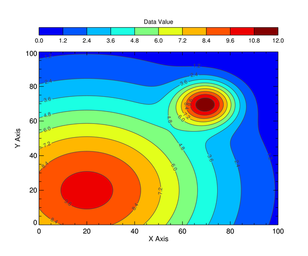
Filled Contour Plot
http://www.idlcoyote.com/gallery/filled_contour_plot_1.png
Several things that are not intuitive and are not explained in the documentation are happening in this one. I cannot precisely reproduce the Coyote version.
PRO Filled_Contour_Plot_FG, WINDOW=window
;Set up variables for the contour plot. Normally, these values
;would be passed into the program as positional and keyword parameters.
minValue = Floor(Min(data))
maxValue = Ceil(Max(data))
nLevels = 10
xtitle = 'X Axis'
ytitle = 'Y Axis'
position = [0.125, 0.125, 0.9, 0.800]
cbposition = [0.125, 0.865, 0.9, 0.895]
cbTitle = 'Data Value'
;Contour Levels
contourLevels = cgConLevels(data, NLevels=10, MinValue=minValue)
;Set up colors for contour plot.
cgLoadCT, 33, NColors=nlevels, Bottom=1, CLIP=[30,255]
TVLCT, palette, /GET
; Open a window and return its reference to the user.
aWindow = Window(WINDOW_TITLE="Filled Contour Plot")
;Draw the filled contour plot.
; - RGB_Table=33 works and creates a discretely filled contour plot. However,
; the TAPER keyword in Colorbar seems to need a non-continuous color pallete
; to not be ignored. Attept to use a reduced color palette failed.
fgC_Fill = Contour(data, /Current, /FILL, C_Value=contourLevels, RGB_Table=palette, $
XTitle=xtitle, YTitle=ytitle, Position=position)
;Must overplot another contour to get the lines.
; - Orientation of the labels is rotated 180 degrees.
; - Must supply own Text() or Symbol() object and use the
; C_Use_Label_Orientation and C_Label_Objects keywords to get proper orientation.
fgC_Lines = Contour(data, C_Value=contourLevels, OverPlot=fgC_Fill, C_Label_Show=1)
;Add the right and top axes
; In IDL 8.2.3+ set Location='Right' or 'Top' and skip finding [xy]range.
IF Float(!Version.Release) GE 8.3 THEN BEGIN
xrange = (fgC_Fill.Axes)[0].Range
yrange = (fgC_Fill.Axes)[1].Range
xAxis = Axis('X', Target=fgC_Fill, Location=[xrange[1], $
yrange[1], 0], TickFormat='(A1)', TickDir=1)
yAxis = Axis('Y', Target=fgC_Fill, Location=[xrange[1], $
yrange[0], 0], TickFormat='(A1)', TickDir=1)
ENDIF ELSE BEGIN
xAxis = Axis('X', Target=fgC_Fill, Location='Right', $
TickFormat='(A1)', TickDir=1)
yAxis = Axis('Y', Target=fgC_Fill, Location='Top', $
TickFormat='(A1)', TickDir=1)
ENDELSE
;Add the colorbar
; - The title and ticklabels are always on the same side. Try to use an Axis() instead
; - The Taper keyword is ignored: It is suppose to be ignored if the color table
; is continuous, but here, "palette" is reduced... Perhaps data is out of range? Do not see how...
; - TickFormat is ignored
fgCB = Colorbar(Target=fgC_Fill, Position=cbPosition, Title='Data Value', Taper=0, $
Border=1, TextPos=1, TickFormat='(A1)')
;Create an axis for the colorbar to try and put the ticklabels on the bottom.
; - It seems as though axes cannot have colorbars as targets...
; - cbAxis is undefined after attempt
; - No information is given as to what happened...
cbAxis = Axis('X', Target=fgCB, Location=[cbPosition[0:1], 0], Axis_Range=[minValue, maxValue])
END ;*********************************************************** ******
; This main program shows how to call the program and produce
; various types of output.
; Display the plot in a resizeable graphics window.
Filled_Contour_Plot_FG, Window=window
; Create a PostScript file. Linestyles are not preserved in IDL 8.2.3 due
; to a bug. Only encapsulated PostScript files can be created.
window.save, 'filled_contour_plot_fg.eps'
; Create a PNG file with a width of 600 pixels. Resolution of this
; PNG file is not very good.
window.save, 'filled_contour_plot_fg.png', WIDTH=600
; For better resolution PNG files, make the PNG full-size, then resize it
; with ImageMagick. Requires ImageMagick to be installed.
window.save, 'filled_contour_plot_fg_fullsize.png'
Spawn, 'convert filled_contour_plot_fg_fullsize.png -resize 600 filled_contour_plot_fg_resized.png'
END
|
|
|
|
| Re: cgGallery with function graphics [message #87832 is a reply to message #87787] |
Thu, 27 February 2014 12:15 |
Matthew Argall
Messages: 286
Registered: October 2011
|
Senior Member |
|
|
Image with Contours Overlayed
http://www.idlcoyote.com/gallery/image_plot_with_contours.pn g
More problems/bugs/not-intuitive-things with this one that I could not solve. My two attempts are below.
PRO Image_With_Contours_Overlayed_FG, WINDOW=aWindow
; Example Gaussian data.
img = cgDemoData(26)
; Set up variables for the contour plot. Normally, these values
; would be passed into the program as positional and keyword parameters.
minValue = Floor(Min(image))
maxValue = Ceil(Max(image))
nLevels = 10
xtitle = 'X Axis'
ytitle = 'Y Axis'
position = [0.125, 0.125, 0.9, 0.800]
cbposition = [0.125, 0.865, 0.9, 0.895]
cbTitle = 'Data Value'
;Contour levels
contourLevels = cgConLevels(img, NLevels=10, MinValue=minValue)
; Set up colors for contour plot.
cgLoadCT, 33, CLIP=[30,255]
tvLCT, palette, /Get
;APPROACH 1: Plot the image directly (does not work)
; The data coordinates are tied to the dimensions of the image. Setting [XY]Range
; will select a subwindow of the image (a 10x200 strip). Setting Image_Location and
; Image_Dimensions allows you to squeeze the entire image into the thin strip. There
; is no natural way to then set the size of the image to something normal without
; clicking on the image and stretching it.
fgImage1 = Image(img, XRange=[10,20], YRange=[-100,100], RGB_Table=palette, $
Position=position, Axis_Style=1, Image_Location=[10,-100], $
Image_Dimensions=[10,200])
; Open a window and return its reference to the user.
aWindow = Window(WINDOW_TITLE="Image with Contours Overlayed")
;APPROACH 2: Paste the image into a set of axes
; Because the axes are fixed to the image's dimensions, setting the Overplot keyword
; results in the same behavior as described above. Here, I will play with the Image's
; aspect ratio to fit it inside the axes.
fgPlot = Plot([10,20], [-100,100], /Current, /NoData, XStyle=1, YStyle=1, $
Xtitle=xtitle, YTitle=ytitle, Position=position)
;Must set the aspect ratio in order to fill out the axes, otherwise
coords = fgPlot -> ConvertCoord(position[[0,2]], position[[1,3]], /Normal, /To_Device)
aspect = double(coords[1,1]-coords[1,0]) / double(coords[0,1]-coords[0,0])
;Create the image
; - The image does not stay fitted to the axes if the window is resized.
; The Aspect_Ratio would have to be updated each time.
fgImage = Image(img, Aspect_Ratio=aspect, Position=position, /Current, RGB_Table=palette)
;Bring the plot forward so that the tickmarks are on top.
fgPlot -> Order, /Bring_Forward
;Create the contours
; - Labels are still up-side-down. See the C_Label_Objects and C_Use_Label_Orientation
fgContour = Contour(img, C_Value=contourLevels, C_Color='Dark Grey', Overplot=fgPlot, $
C_Label_Show=1)
;Create the colorbar
; - Generates error: "% Attempt to call undefined method: 'IDLITSYMBOL::GETVISUALIZATIONS'."
; but still creates the colorbar
; - fgCB is undefined after the call
fgCB = Colorbar(Target=fgImage, Position=cbPosition, TextPos=1, Title='Data Value')
END ;*********************************************************** ******
; This main program shows how to call the program and produce
; various types of output.
; Display the plot in a resizeable graphics window.
Image_With_Contours_Overlayed_FG, Window=window
; Create a PostScript file. Linestyles are not preserved in IDL 8.2.3 due
; to a bug. Only encapsulated PostScript files can be created.
window.save, 'image_with_contours_overlayed_fg.eps'
; Create a PNG file with a width of 600 pixels. Resolution of this
; PNG file is not very good.
window.save, 'image_with_contours_overlayed_fg.png', WIDTH=600
; For better resolution PNG files, make the PNG full-size, then resize it
; with ImageMagick. Requires ImageMagick to be installed.
window.save, 'image_with_contours_overlayed_fg_fullsize.png'
Spawn, 'convert image_with_contours_overlayed_fg_fullsize.png -resize 600 image_with_contours_overlayed_fg_resized.png'
END
|
|
|
|
|
|
|
|
|
|
|
|
| Re: cgGallery with function graphics [message #87837 is a reply to message #87834] |
Thu, 27 February 2014 12:54 |
David Fanning
Messages: 11724
Registered: August 2001
|
Senior Member |
|
|
David Fanning writes:
> I can't even get this one to compile. Doesn't like [XY]Range or Aspect
> keywords to the Image function, it looks like.
OK, I see the problem. When I put a Compile_Opt idl2 in the code, then I
found this error:
minValue = Floor(Min(image))
maxValue = Ceil(Max(image))
This should be:
minValue = Floor(Min(img))
maxValue = Ceil(Max(img))
Actually, now I see the real colors! Progress, I suppose. The image
window is not so bad, actually. I wonder if that error at the start of
your program was causing some of the other grief you were experiencing?
Cheers,
David
--
David Fanning, Ph.D.
Fanning Software Consulting, Inc.
Coyote's Guide to IDL Programming: http://www.idlcoyote.com/
Sepore ma de ni thue. ("Perhaps thou speakest truth.")
|
|
|
|
|
|
| Re: cgGallery with function graphics [message #87878 is a reply to message #87787] |
Sat, 01 March 2014 17:38 |
Matthew Argall
Messages: 286
Registered: October 2011
|
Senior Member |
|
|
Filled Area Plot
http://www.idlcoyote.com/gallery/filled_area_plot.png
PRO Filled_Area_Plot_FG, WINDOW=awindow
compile_opt strictarr
; Set up variables for the plot. Normally, these values would be
; passed into the program as positional and keyword parameters.
x = Findgen(101)
y = 4 * Sin(x * !DtoR) / Exp( (x-15) / 25.)
; Set up the low and high x indices of the area under the curve
; you want to fill.
low = 20
high = 45
; Find the y indices associated with the low and high indices.
lowY = 4 * Sin(low * !DtoR) / Exp( (low-15) / 25.)
highY = 4 * Sin(high * !DtoR) / Exp( (high-15) / 25.)
indices = Value_Locate(x, [low, high])
lowIndex = indices[0]
highIndex = indices[1]
; Make sure the indices you find correspond the the right X indices.
IF x[lowIndex] LT low THEN lowIndex = lowIndex + 1
IF x[highIndex] GT high THEN highIndex = highIndex - 1
; Open a window and return its reference to the user.
aWindow = Window(WINDOW_TITLE="Filled Area Plot")
;
;APPROACH 1:
; Similar to the Coyote example, create a plot, then fill it with a polygon.
;
; Draw the plot axes.
fgPlot = Plot(x, y, /Current, XTitle='X Axis', YTitle='Y Axis', Color='red', $
Name='4*Sin(x) $\slash$ e^(x-15) $\slash$ 25', LAYOUT=[1,2,1], $
Title='Example Using Polygon')
; Create closed polygons to color fill.
yMin = fgPlot.yrange[0]
xpoly = [ low, low, x[lowIndex:highIndex], high, high]
ypoly = [yMin, lowY, y[lowIndex:highIndex], highY, yMin]
; Create a filled polygon and keep it in the data space.
fgPoly = Polygon(xpoly, ypoly, /Data, Target=fgPlot, /Fill_Background, $
Fill_Color='Dodger Blue', Name='Area Under Plot')
; Bring the plot to the front
fgPlot -> Order, /Bring_Forward
;
;APPROACH 2:
; Using the FILL_* keywords in the Plot function. This does not reproduce the
; Coyote example, but it illustrates another manner of filling the area under
; the plot with a polygon. Adjust Fill_Level to see what happens.
;
; It would be nice if there were Fill_XRange and Fill_YRange keywords.
;
; Draw the plot axes and fill the area below it.
fgPlot = Plot(x, y, /Current, XTitle='X Axis', YTitle='Y Axis', Color='red', $
Name='4*Sin(x) $\slash$ e^(x-15) $\slash$ 25', $
/Fill_Background, Fill_Color='Dodger Blue', Fill_Level=0.3, $
Layout=[1,2,2], Title='Example using Fill_* Keywords (Fill_Level=0.3)')
END ;*********************************************************** ******
; This main program shows how to call the program and produce
; various types of output.
; Display the plot in a resizeable graphics window.
Fill_Area_Plot_FG, Window=window
; Create a PostScript file. Linestyles are not preserved in IDL 8.2.3 due
; to a bug. Only encapsulated PostScript files can be created.
window.save, 'filled_area_plot_fg.eps'
; Create a PNG file with a width of 600 pixels. Resolution of this
; PNG file is not very good.
window.save, 'filled_area_plot_fg.png', WIDTH=600
; For better resolution PNG files, make the PNG full-size, then resize it
; with ImageMagick. Requires ImageMagick to be installed.
window.save, 'filled_area_plot_fg_fullsize.png'
Spawn, 'convert filled_area_plot_fg_fullsize.png -resize 600 filled_area_plot_fg_resized.png'
END
|
|
|
|
| Re: cgGallery with function graphics [message #87879 is a reply to message #87787] |
Sat, 01 March 2014 17:39 |
Matthew Argall
Messages: 286
Registered: October 2011
|
Senior Member |
|
|
Filled Area By Height Plot
http://www.idlcoyote.com/gallery/height_filled_area_plot.pro
PRO Filled_Area_By_Height_Plot_FG, WINDOW=awindow
compile_opt strictarr
; Set up variables for the plot. Normally, these values would be
; passed into the program as positional and keyword parameters.
x = Findgen(101)
y = 4 * Sin(x * !DtoR) / Exp( (x-15) / 25.)
; Set up the low and high x indices of the area under the curve
; you want to fill.
low = 10
high = 45
; Find the y indices associated with the low and high indices.
lowY = 4 * Sin(low * !DtoR) / Exp( (low-15) / 25.)
highY = 4 * Sin(high * !DtoR) / Exp( (high-15) / 25.)
indices = Value_Locate(x, [low, high])
lowIndex = indices[0]
highIndex = indices[1]
; Make sure the indices you find correspond the the right X indices.
IF x[lowIndex] LT low THEN lowIndex = lowIndex + 1
IF x[highIndex] GT high THEN highIndex = highIndex - 1
; Open a window and return its reference to the user.
aWindow = Window(WINDOW_TITLE="Filled Area by Height Plot")
; Turn refresh off until we are finished adding all of the graphics
aWindow -> Refresh, /Disable
; Draw the plot axes.
fgPlot = Plot(x, y, /Current, XTitle='X Axis', YTitle='Y Axis', Color='Navy', $
Name='4*Sin(x) $\slash$ e^(x-15) $\slash$ 25')
;APPROACH 1
; - Use a bunch of polygons to fill the area under the curve. Necessary for
; versions of IDL < 8.2.1
IF (!Version.Release LE 8.2) THEN BEGIN
; Scale the y data for colors.
cgLoadCT, 4, /Brewer, Clip=[50, 230], RGB_Table=RGB_Table
; Draw the area under the curve with scaled colors.
min_y = Min(y[lowIndex:highIndex], Max=max_y)
colors = BytScl(y, MIN=min_y, MAX=max_y)
; Number of polygons to make
nPoly = highIndex-lowIndex
; Create the polygons
fgPolygons = objarr(nPoly)
FOR j=lowIndex,highIndex-1 DO BEGIN
;Each little area has to be its own color/polygon. Create the vertices.
xpoly = [x[j], x[j], x[j+1], x[j+1], x[j]]
ypoly = [!Y.CRange[0], y[j], y[j+1], !Y.CRange[0], !Y.CRange[0]]
;Create the polygon
fgPolygons[j-lowIndex] = Polygon(xpoly, ypoly, /Data, Target=fgPlot, $
LineStyle=6, /Fill_Background, $
Fill_Color=reform(RGB_Table[colors[j],*]), $
Name='Filled Area' + strtrim(j-lowIndex))
ENDFOR
;APPROACH 2
; - Use the Vert_Colors and RGB_Table keywords (introduced in IDL 8.2.1)
; - Cannot test because I have IDL 8.2
ENDIF ELSE BEGIN
; Create closed polygons to color fill.
yMin = fgPlot.YRange[0]
xpoly = [ low, low, x[lowIndex:highIndex], high, high]
ypoly = [yMin, lowY, y[lowIndex:highIndex], highY, yMin]
;Get the color table
cgLoadCT, 4, /Brewer, RGB_Table=RGB_Table
;Create an array of indices between 50 and 230, scaled by height.
; - The RGB_Table keyword in Polygon takes a full palette [256x3], so I
; presume giving a smaller palette will not work.
colors = BytScl(y, MIN=min_y, MAX=max_y, Top=256-76) + 50B
;Create a filled polygon and keep it in the data space.
; - I assume the Vert_Colors keyword will color the area between each
; vertice the correct color...
fgPoly = Polygon(xpoly, ypoly, /Data, Target=fgPlot, /Fill_Background, $
Fill_Color='Dodger Blue', Name='Area Under Plot', $
RGB_Table=RGB_Table, Vert_Color=colors, LineStyle=6)
ENDELSE
;Add lines at the edges of the filled region
yrange = fgPlot.YRange
fgLine1 = PolyLine([low, low], [yrange[0], lowY], /Data, Target=fgPlot, Color='Grey', $
Name='Low Line')
fgLine2 = PolyLine([high, high], [yrange[0], highY], /Data, Target=fgPlot, Color='Grey', $
Name='High Line')
; Bring the plot to the front
fgPlot -> Order, /Bring_To_Front
;Refresh the plot
aWindow -> Refresh
END ;*********************************************************** ******
; This main program shows how to call the program and produce
; various types of output.
; Display the plot in a resizeable graphics window.
Filled_Area_By_Height_Plot_FG, Window=window
; Create a PostScript file. Linestyles are not preserved in IDL 8.2.3 due
; to a bug. Only encapsulated PostScript files can be created.
window.save, 'filled_area_by_height_plot_fg.eps'
; Create a PNG file with a width of 600 pixels. Resolution of this
; PNG file is not very good.
window.save, 'filled_area_by_height_plot_fg.png', WIDTH=600
; For better resolution PNG files, make the PNG full-size, then resize it
; with ImageMagick. Requires ImageMagick to be installed.
window.save, 'filled_area_by_height_plot_fg_fullsize.png'
Spawn, 'convert filled_area_by_height_plot_fg_fullsize.png -resize 600 filled_area_by_height_plot_fg_resized.png'
END
|
|
|
|
|
|
| Re: cgGallery with function graphics [message #87881 is a reply to message #87880] |
Sat, 01 March 2014 17:54 |
David Fanning
Messages: 11724
Registered: August 2001
|
Senior Member |
|
|
David Fanning writes:
>
> Matthew Argall writes:
>
>> Filled Area Plot
>> http://www.idlcoyote.com/gallery/filled_area_plot.png
>
> After I fix the name in the main-level program, this program fails for
> me (IDL 8.2.3) with this error message:
>
> % Subscripts are not allowed with object properties.
> % Execution halted at: FILLED_AREA_PLOT_FG 39 C:\IDL
> \filled_area_plot_fg.pro
> % $MAIN$ 71 C:\IDL
> \filled_area_plot_fg.pro
>
> This is the line it is failing on.
>
> ; Create closed polygons to color fill.
> --->>> yMin = fgPlot.yrange[0]
I fixed this error like this:
; Create closed polygons to color fill.
yrange = fgPlot.yrange
yMin = yrange[0]
Runs, OK, now.
Cheers,
David
--
David Fanning, Ph.D.
Fanning Software Consulting, Inc.
Coyote's Guide to IDL Programming: http://www.idlcoyote.com/
Sepore ma de ni thue. ("Perhaps thou speakest truth.")
|
|
|
|
 comp.lang.idl-pvwave archive
 Members
 Search
 Help
Help Login
Login Home
Home


")
