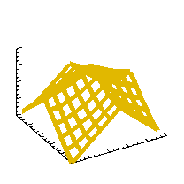
Folks,
OK, forget labeling the color bar. I can live without
that.
I would consider the week a triumph if someone could just
explain to me, like I was a 10 year old child, how to
use the IDL 8.1 contour function to produce a contour
plot with four colors of my choosing. The colors will
be used like this:
Data between 0.00 and 0.25 should be red.
Data between 0.25 and 0.50 should be blue.
Data between 0.50 and 0.75 should be green.
Data between 0.75 and 1.00 should be yellow.
Here is the program I am trying to run, using some
ideas from Mark Piper's program from yesterday.
You see two different ways of trying to get the
Colorbar() colors right. One of which actually
works. But neither of the Contour() plots have
the right colors. The Coyote Graphics plot at the
end is what I am trying to achieve.
PRO ContourTest
; Create a simple, random dataset for contouring:
data = RANDOMU(-3L, 9, 9)
LoadCT, 0
TVLCT, 255, 0, 0, 0
TVLCT, 0, 0, 255, 1
TVLCT, 0, 255, 0, 2
TVLCT, 255, 255, 0, 3
TVLCT, rr, gg, bb, /GET
rgb = Transpose([[rr[0:3]],[gg[0:3]],[bb[0:3]]])
Help, rgb
rgb = Congrid(rgb, 3, 256)
levels =[0.0, 0.25, 0.5, 0.75]
; Contour function try 1.
w1 = Window(DIMENSIONS=[500, 400])
ctr=contour(data, /CURRENT, C_VALUE=levels, $
POSITION=[0.1, 0.1, 0.9, 0.8], /FILL, $
RGB_TABLE=rgb, $
AXIS_STYLE=2)
names = String(levels,FORMAT='(F0.2)')
cb = Colorbar(TARGET=ctr, $
POSITION=[0.1, 0.85, 0.9, 0.9])
rgb = Transpose([[rr[0:3]],[gg[0:3]],[bb[0:3]]])
Help, rgb
; Contour function try 2.
w2 = Window(DIMENSIONS=[500, 400])
ctr=contour(data, /CURRENT, C_VALUE=levels, $
POSITION=[0.1, 0.1, 0.9, 0.8], /FILL, $
RGB_TABLE=rgb, RGB_INDICES=Indgen(4), $
AXIS_STYLE=2)
names = String(levels,FORMAT='(F0.2)')
cb = Colorbar(TARGET=ctr, $
POSITION=[0.1, 0.85, 0.9, 0.9])
; Coyote graphics.
cgWindow, WXSize=500, WYSize=400
cgContour, data, LEVELS=levels, C_COLORS=Indgen(4), $
POSITION=[0.1, 0.1, 0.9, 0.8], /FILL, /ADDCMD
cgColorBar, NCOLORS=4, RANGE=[0,1], FORMAT='(F0.2)', $
DIVISIONS=4, /FIT, /ADDCMD
END
If you can get this to me before Nadal beats Roddick,
you will get bonus credit, which can be used to ask
function graphics questions at some time in the future. ;-)
Cheers,
David
--
David Fanning, Ph.D.
Fanning Software Consulting, Inc.
Coyote's Guide to IDL Programming: http://www.dfanning.com/
Sepore ma de ni thui. ("Perhaps thou speakest truth.")
|
 comp.lang.idl-pvwave archive


 Members
 Search
 Help
Help Login
Login Home
Home


