
Filtering Images in the Frequency Domain
QUESTION: I've heard about frequency domain filtering of images. How can I build image filters and do this in IDL?
![]()
ANSWER: Filtering in the frequency domain is a common image and signal processing technique. It can smooth, sharpen, de-blur, and restore some images.
There are three basic steps to frequency domain filtering:
- The image must be transformed from the spatial domain into the frequency domain using the Fast Fourier transform.
- The resulting complex image must be multiplied by a filter (that usually has only real values).
- The filtered image must be transformed back to the spatial domain.
These steps can be implemented in IDL using the Fast Fourier transform function FFT. A -1 argument to the FFT function indicates a transformation from the spatial to the frequency domain, and a 1 indicates the reverse transformation. The general form of the command is written like this, where image is either a vector or a two-dimensional image and filter is a vector or two-dimensional array designed to filter out certain frequencies in the image:
filtered_image = FFT(FFT(image, -1) * filter, 1)
![]()
Building Image Filters
IDL makes it easy to build many types of image filters with its array-oriented operators and functions. Many common filters take advantage of what is called a frequency image or Euclidean distance map. An Euclidean distance map for a two-dimensional image is an array of the same size as the image. Each pixel in the distance map is given a value that is equal to its distance from the nearest corner of the two-dimensional array. The DIST command in IDL is used to create the Euclidean distance map or frequency image. For example, to see a surface representation of a simple distance map, type:
SURFACE, DIST(40)
A common type of filter to use in frequency domain filtering is a Butterworth frequency filter. The general form of a low-pass Butterworth frequency filter is given by this equation:
filter = 1 / [1 + C(R/Ro)^2n]
Here the constant C is set equal to 1.0 or 0.414 (the value defines the magnitude of the filter at the point where R=Ro as either 50% or 1/Sqrt(2)), R is the frequency image, Ro is the nominal filter cutoff frequency (represented as a pixel width in practice), and n is the order of the filter and is usually 1.
A high-pass Butterworth frequency filter is given by this equation:
filter = 1 / [1 + C(Ro/R)^2n]
To see how frequency domain filtering works, open the image file convec.dat, which is among the files Research Systems provides with its demonstation directories. Your code will look something like this. (Click here to download the entire example IDL code.)
   file = FILEPATH('convec.dat', SUBDIR='training')
   OPENR, lun, file, /GET_LUN
   convec = BYTARR(248,248)
   READU, lun, convec
   FREE_LUN, lun
Open a large window, load a color table, and display the unprocessed image in the upper left-hand corner, like this:
   WINDOW, 0, XSIZE=248*2, YSIZE=248*2
   LOADCT, 13
   TV, convec, 0
Transforming the Image into the Frequency Domain
The first step in frequency domain filtering is to transform the image from the spacial domain into the frequency domain with the FFT function, like this:
freqDomainImage = FFT(convec, -1)
In general, the low frequency terms usually represent the general shape of the image and the high frequency terms are needed to sharpen the edges and provide fine detail. Looking at the frequency domain image is not usually instructive, but it is sometimes useful to observe the power spectrum of the frequency domain image.
The power spectrum is a plot of the magnitude of the various components of the frequency domain image. Different frequencies are represented at different distances from the origin (usually represented as the center of the image) and different directions from the origin represent different orientations of features in the original image. The power at each location shows how much of that frequency and orientation is present in the image. The power spectrum is particularly useful for isolating periodic structures or noise in the image. The power spectrum magnitude is usually represented on a log scale, since power can vary dramatically from one frequency to the next.
To see the power spectrum of this image next to the image, type:
   power = SHIFT(ALOG(ABS(freqDomainImage)), 124, 124)
   power = power - Min(power)
   power = power * (255.0/Max(power))
  TV, power, 1
You can see from the power spectrum that this image has lots of periodic structure at increasing frequencies. (Your display screen should look similar to the illustration below.) The next step will filter out the higher frequencies.
Appling the Frequency Domain Filter
The next step in the frequency domain filtering of an image is to apply a filter to the frequency domain image. Here you are going to construct a Butterworth low-pass frequency filter. This will filter out the high image frequencies that give detail to the image, and will result in an image smoothing operation. Construct the filter by typing:
filter = 1.0 / ( 1.0d + (DIST(248)/15.0)^2 )
Notice that the cutoff frequency width is 15 pixels here. You will be eliminating about half of the higher frequencies that you see in the power spectrum in the illustration below. These frequencies are normally those that provide detail in an image.
To apply the filter, back transform the image from the frequency domain to the spacial domain, and display the filtered image, type:
   filtered = FFT(freqDomainImage * filter, 1)
   TV, filtered, 2
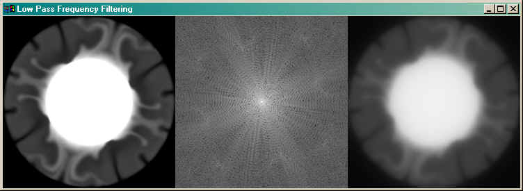
Your display screen should look similar to the illustration below. The original image is on the left. The power spectrum of the original image is shown in the middle. Notice that there is a lot of periodic structure in this image. The filtered image is shown on the right. A low pass filter tends to blur or smooth the image, since it is the high frequency components that give the image detail.
![]()
Last Updated 6 March 2003