
Navigating GOES Images
QUESTION: I have downloaded a GOES image of Peru in TIFF format. With this image, I have downloaded navigation files that specify the latitude and longitude for each pixel in the image. (These are calculated by the data provider from the GVAR file that is downloaded with the raw image data.) Since GOES images are not projected into any map projection, what I would like to do is project this image into a map projection and save it along with its map information in a format that I can use in ENVI. I was hoping I could create a geoTIFF file from the information I have. Can you help?
![]()
ANSWER: You are correct that GOES images are not projected. And, as Mark Conner points out, to do a proper job of projecting them requires access to the GVAR navigation stream that is downloaded with the raw image data. Some low-level IDL files (the tarball near the bottom of the page) are provided for this purpose.
But you won't need those here. The navigation files you have were generated by the data provider from the GVAR data, so we can just use those to create a projected map image. I have downloaded a suitable image and navigation file, and it was easy enough to read those in the normal IDL way. I have created three variables, peruimage, peru_lat, and peru_lon, and saved these in an IDL save file for people who wanted to follow along with this discussion (2.2 MB). I have rebinned the original data (which was 1200x862) to half its size (600x431) to save bandwidth. This does not effect the results. The image is byte data, scaled from 0 to 255, and the navigation arrays are long integers, that must be divided by 10000 to restore their original values. Download the save file and type these IDL commands. Or, you can simply run the GOES_Example program to run though the following commands automatically. (Other programs from the Coyote Library are also required.)
Please note that the procedure described here can be done much more simply with the Coyote Library mapping routine cgWarpToMap. Please see the article Mapping Data Associated with Lat/Lon Arrays for a faster way of creating the graphics display outlined here. Other examples of navigating GOES images can be found in the Coyote Plot Gallery.
    filename = 'goes_example_data.sav'     Restore, filename
    peru_lat = Temporary(peru_lat) / 10000.
    peru_lon = Temporary(peru_lon) / 10000.
    Help, peruimage, peru_lat, peru_lon
         PERUIMAGE       BYTE      = Array[600, 431]
         PERU_LAT        FLOAT     = Array[600, 431]
         PERU_LON        FLOAT     = Array[600, 431]
We will need to know the center of this image of the map projection, so we find it like this.
     s = Size(peruimage, /DIMENSIONS)
    center_lat = peru_lat[s[0]/2, s[1]/2]
    center_lon = peru_lon[s[0]/2, s[1]/2]
The image is 600 by 431 in size, and the center latitude is -3.01190 degrees and the center longitude is -75.0101 degrees.
The Map_Patch command in IDL will take a longitude and latitude array and an image, and will warp the image into the map projection. But, in order to do so, a map projection space must first be created with the cgMap_Set command. In the case of doing this on the display, this means a graphics window must first be opened so cgMap_Set can fit a map coordinate space into it. We prepare for the cgMap_Set command with these commands.
     cgLoadCT, 0
    cgDisplay, 800, 575, TITLE='GOES Image in Albers Projection', $
            XPOS=20, YPOS=20     cgText, 0.5, 0.5, /NORMAL, FONT=0, ALIGN=0.5, $
           'The image is being warped. Please do not close this window.'
The key to setting up the map projection space properly is to specify, with the Limit keyword, the extent of the image, so that the map projection space is coincident with the image. To do this correctly, we need to use the eight-element version of the Limit keyword, which specifies the left, top, right, and bottom sides of the image, rather than the four-element version of the Limit keyword, which specifies the location of two opposite corners of the image. The code to locate the image sides is straightforward.
     lon_cindex = s[0]/2 ; Center longitude
    lat_cindex = s[1]/2 ; Center latitude      ; Longitude sides.
    left_lon = peru_lon[0, lat_cindex]
    top_lon = peru_lon[lon_cindex, s[1]-1]
    right_lon = peru_lon[s[0]-1, lat_cindex]
    bottom_lon = peru_lon[lon_cindex, 0]      ; Latitude sides.
    left_lat = peru_lat[0, lat_cindex]
    top_lat = peru_lat[lon_cindex, s[1]-1]
    right_lat = peru_lat[s[0]-1, lat_cindex]
    bottom_lat = peru_lat[lon_cindex, 0]
The sides of the image, in longitude and latitude, respectively for the left, top, right, and bottom sides are these.
   -97.5555     -75.0104    -52.5493     -75.0108    -3.05290      12.7496
   -3.05250     -19.1563
If we do the same thing for the corners of the image, we find the corners of the image, starting in the uppper left and proceeding clockwise to be these.
   -98.2703      12.9336    -51.8385      12.9320    -50.8345     -19.4527
   -99.2801     -19.4555
Now we are ready to create the map projection space. I am going to use an Albers Equal Area Conic projection. I use cgMap_Set and the Limit keyword to set it up.
    cgMap_Set, center_lat, center_lon, /Albers, /NOBORDER, $
      STANDARD_PARALLEL=[-19, 21], /NOERASE, POSITION=[0,0,1,1], $
      LIMIT=[left_lat,  left_lon,  top_lat,    top_lon, $
             right_lat, right_lon, bottom_lat, bottom_lon], $
Finally, we are ready to do the warping of the image with Map_Patch. At the same time, we are going to warp the latitude and longitude arrays. We pass all three arrays to Map_Patch, like this.
    warp = Map_Patch(peruimage, peru_lon, peru_lat)
   warp_lat = Map_Patch(peru_lat, peru_lon, peru_lat)
   warp_lon = Map_Patch(peru_lon, peru_lon, peru_lat)
Here is where you have to be careful. Warping the latitude and longitude arrays can result in all kinds of artifacts and strange values in the output array. Be very careful in processing the results. Make sure what you do next makes sense to you. For example, in this warping I found a great many array values of zero, especially around the edge of the warped arrays. So much so that rather than "fix" the warped arrays, I decided to just abandon a one-pixel strip about the outside of the warped image. I trimmed the arrays like this.
[Editor's Note: I did discover that most of this strangeness in the warping process will go away if you set the TRIANGULATE keyword to Map_Patch. This gave me good values around the edges of the warped arrays, although there were still "missing" data points in the very center of the arrays. My advice would be to use the TRIANGULATE keyword, but take great care if you are using values in the warped arrays near the center of the map projection.]
     s = Size(warp, /DIMENSIONS)
    warp =         warp[1:s[0]-2, 1:s[1]-2]
    warp_lat = warp_lat[1:s[0]-2, 1:s[1]-2]
    warp_lon = warp_lon[1:s[0]-2, 1:s[1]-2]
    center_lat = warp_lat[s[0]/2, s[1]/2]
    center_lon = warp_lon[s[0]/2, s[1]/2]
After this trimming, I again find the side points of the warped image.
     s = Size(warp, /DIMENSIONS)          ; Side of warped image.
    left_lon = warp_lon[0, lat_cindex]
    top_lon = warp_lon[lon_cindex, s[1]-1]
    right_lon = warp_lon[s[0]-1, lat_cindex]
    bottom_lon = warp_lon[lon_cindex, 0]
    left_lat = warp_lat[0, lat_cindex]
    top_lat = warp_lat[lon_cindex, s[1]-1]
    right_lat = warp_lat[s[0]-1, lat_cindex]
    bottom_lat = warp_lat[lon_cindex, 0]
The sides of the warped image are located here.
   -97.470690      -80.650603    -52.690633      -80.593828
   -7.0329920       12.633804    -7.0321833      -19.102513
And if I also determine and print out the corners of the warped image, I find them here.
    -97.613224       12.572246
   -52.548995       12.573068    -52.775074      -19.165249
   -97.385715      -19.166099
Now, all I have to do is re-execute my cgMap_Set command, with the warped image limit and center, display the image, and add boundaries and grids with cgMap_Continents and cgMap_Grid. The code looks like this.
    cgMap_Set, center_lat, center_lon, /Albers, /NOBORDER, $
        STANDARD_PARALLEL=[-19, 21], POSITION=[0,0,1,1], $
        LIMIT=[left_lat, left_lon, top_lat, top_lon, $
               right_lat, right_lon, bottom_lat, bottom_lon], /NOERASE
    cgImage, warp     cgMap_Continents, COLOR='Pale Goldenrod', /HIRES
    cgMap_Continents, /COUNTRIES, COLOR='Pale Goldenrod', /HIRES
    cgMap_Grid, /LABEL, COLOR='Light Gray'
The output of these commands is shown in the figure below.
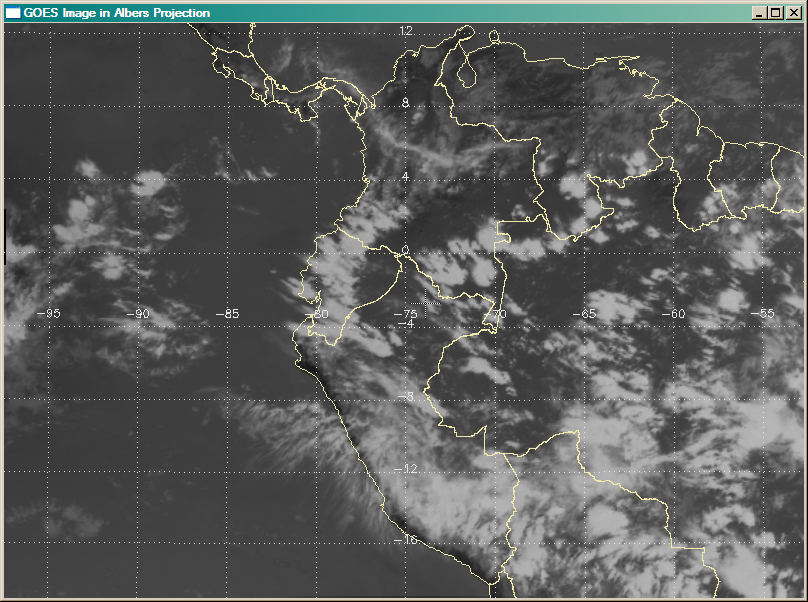 |
| The GOES image warped into an Albers Equal Area Conic map projection. |
![]()
Creating a GeoTIFF File from the Map-Projected Image
The next step is to create map projection information in such a form that it can be either conveyed directly to ENVI or stored in something like a GeoTIFF file. In either case, we need map information in the Cartesian grid space (sometimes called the UV space). You can think of this space as a sort of graph paper we draw the datum locations on, before the locations are transformed into the latitude and longitude values of the map projection. The Map_Proj_Forward command in IDL is use to convert latitude and longitude values to this Cartesian grid space. But, of course, we need to create a map structure, containing map projection information, with Map_Proj_Init before we can use Map_Proj_Forward. Map_Proj_Init is similar to Map_Set in this respect, except that Map_Proj_Init does not give us the ability to use an eight-element Limit array.
The code to set up the Albers Equal Area Conic map projection and warp the sides of the image in UV space is here.
      alberMap = MAP_PROJ_INIT('Albers Equal Area Conic', $
       DATUM=8, $ ; WGS84        CENTER_LAT=center_lat, $
       CENTER_LON=center_lon, $        STANDARD_PAR1=-19, $
       STANDARD_PAR2=20)
    ; We want to transform the sides of the image from lat/lon to UV space.
    uv = MAP_PROJ_FORWARD([left_lon, top_lon, right_lon, bottom_lon], $
                          [left_lat, top_lat, right_lat, bottom_lat], $
                          MAP_STRUCTURE=alberMap)
If we print out the sides of the warped image in UV coordinates, we get this.
    -2361109.5      -468647.94    -592158.50       1837085.2
    2343373.7      -468610.27    -589179.93      -1855137.0
With these values and the size of the warped image, we can then calculate the image scales in both the X and Y directions (these are also called the U and V directions). These scales are normally in meters per pixel. The tie-point is the location of the upper-left corner of the image (assuming the image (0,0) point is in the upper-left, as well). The code looks like this.
     s = Size(warp, /DIMENSIONS)
    xscale = Abs(uv[0,0] - uv[0,2]) / (s[0] )
    yscale = Abs(uv[1,1] - uv[1,3]) / (s[1])     tp = [uv[0,0], uv[1,1]]
The XScale is equal to 5895.3423, the YScale is equal to 6443.6687, and the tie-point is located at (-2361109.5, 1837085.2).
We now have all the information we need to make the geotag structure for the GeoTIFF file. (You may need to consult the GeoTIFF documentation page if you are unsure about the definition of the geotags in the following structure.) The code looks like this.
    geotag = { MODELPIXELSCALETAG: [xscale, yscale, 0], $ ; Scales
               MODELTIEPOINTTAG: [ 0, 0, 0, tp, 0], $  ; Tie point
               GTMODELTYPEGEOKEY: 1, $                GTRASTERTYPEGEOKEY: 1, $
               GEOGRAPHICTYPEGEOKEY: 4326, $
               GEOGLINEARUNITSGEOKEY: 9001, $          ; Meters
               GEOGANGULARUNITSGEOKEY: 9102, $
               PROJECTEDCSTYPEGEOKEY: 32767, $
               PROJECTIONGEOKEY: 32767, $
               PROJCOORDTRANSGEOKEY: 11, $             ; Albers Equal Area Conic
               PROJLINEARUNITSGEOKEY: 9001, $
               PROJSTDPARALLEL1GEOKEY: -19.00000, $
               PROJSTDPARALLEL2GEOKEY: 21.000000, $
               PROJNATORIGINLONGGEOKEY: center_lon, $  ; Center longitude
               PROJNATORIGINLATGEOKEY: center_lat, $   ; Center latitude
               PROJFALSEEASTINGGEOKEY: 0, $
               PROJFALSENORTHINGGEOKEY: 0 }
The final step is to write the GeoTIFF file. Take care to reverse the Y dimension of the image, so the (0,0) point is in the upper-left of the image, and to store byte data. (Write_TIFF will do the latter automatically, in this case.)
Write_TIFF, 'goes_example.tif', Byte(Reverse(warp, 2)), GEOTIFF=geotag
![]()
Read and Display the GeoTIFF Image
The last procedure, then, is to read and display the GeoTIFF image created from the GOES image, to be sure we can recover the image and display annotations on it. First, we read the GeoTIFF image file. Be sure you obtain the geotag structure. Reversing the Y dimension of the image is something that is almost always required for TIFF images.
    tiffimage = 'goes_example.tif'
    image = Read_Tiff(tiffimage, GEOTIFF=geotag)     image = Reverse(image, 2)
Now, read the tie-point and scales from the geotag structure, and locate the four corners of the image.
    s = Size(image, /Dimensions)
   ; Calculate corner points from GeoTIFF structure obtained from file.
   xscale  = geotag.ModelPixelScaleTag[0]
   yscale  = geotag.ModelPixelScaleTag[1]
   tp      = geotag.ModelTiePointTag[3:4]    xOrigin = tp[0]    yOrigin = tp[1]
   xEnd = xOrigin + (xscale * s[0])    yEnd = yOrigin - (yscale * s[1])
Next, set up an Albers Equal Area Conic map projection and convert the four corners of the image into latitude and longitude values.
    alberMap = MAP_PROJ_INIT('Albers Equal Area Conic', $
       DATUM=8, $ ; WGS84        CENTER_LAT=geotag.PROJNATORIGINLATGEOKEY, $
       CENTER_LON=geotag.PROJNATORIGINLONGGEOKEY, $
       STANDARD_PAR1=geotag.PROJSTDPARALLEL1GEOKEY, $
       STANDARD_PAR2=geotag.PROJSTDPARALLEL2GEOKEY)
    lonlat = MAP_PROJ_INVERSE([xOrigin, xEnd, xEnd, xOrigin], $
                              [yEnd, yEnd, yOrigin, yOrigin], $
                               MAP_STRUCTURE=alberMap)
The longitude and latitude values we obtain are these:
   -97.427758      -19.147710    -52.733240      -19.146690
   -52.507448       12.510946    -97.655259       12.509959
Next, we display the GeoTIFF image in a graphics window.
    s = Size(image, /Dimensions)
    cgDisplay, WID=1, s[0], s[1], TITLE='GeoTiff Output', XPOS=70, YPOS=70
    pos = [0, 0, 1, 1]     cgImage, image, POSITION=pos
Finally, we have to set up a UV data coordinate space for drawing the map annotations. We use the corners of the image to do this. The code looks like this. Notice we pass the Albers map structure created above to cgMap_Continents and cgMap_Grid.
     cgPlot, [xOrigin, xEnd], [yEnd, yOrigin], Position=pos, $
          /Nodata, XStyle=5, YStyle=5, /NoErase
    cgMap_Continents, COLOR='Pale Goldenrod', /HIRES, MAP_STRUCTURE=alberMap
    cgMap_Continents, /COUNTRIES, COLOR='Pale Goldenrod', /HIRES, MAP_STRUCTURE=alberMap
    cgMap_Grid, /LABEL, COLOR='Light Gray', MAP_STRUCTURE=alberMap, $
        LATS=Indgen(10) * 4 + (-20), LONS=Indgen(12) * 5 + (-105)
The final result, shown in the figure below, looks identical to the original warped image. The GeoTIFF image can be opened directly in ENVI if you so desire.
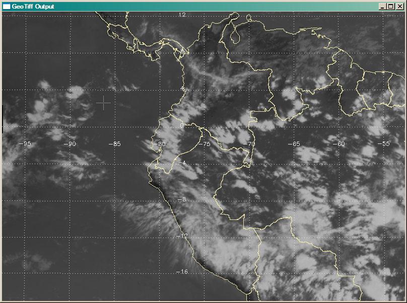 |
| The GeoTIFF image displayed in an Albers Equal Area Conic map projection. |
![]()
Version of IDL used to prepare this article: IDL 7.0.1.
![]()
Copyright © 2008 David W. Fanning
Written: 28 March 2008
Updated: 12 Sept 2012