
Creating GPD Files
QUESTION: A number of tools at the National Snow and Ice Data Center (NSIDC) are used to grid satellite data into a particular map region (e.g., mapx or ms2gt). They all seem to require input of a "GPD" file. I can see that this file blends map projection information with information about the grid I am trying to create, but it is not obvious to me where the grid is located on the map. Or, even more important, how to go about creating a GPD file for a study area of my own. Can you help?
![]()
ANSWER: Typically, when you start a project using satellite data, you start with a portion of the Earth you want to study. It could be the Amazon basin or the Arctic ocean, or even a local county. Wherever it is, the first order of business is to find satellite data that passes over the region and covers it in some way. Sometimes the data only partially covers the area you are interested in. Often you wish to use data from two or more different satellite sensors. (See the last portion of this article for a MODIS example.)
Inevitably, the data you wish to use is available in different map projections (or maybe in raw unprojected swaths) and different resolutions. To make sense of the data, it is necessary to convert all the data to the same map projection and resolution. There are tools available to help with this, and at NSIDC most of the tools require a GPD file to specify both the map projection and the grid location and resolution of your area of interest on that map projection.
Originally at NSIDC two files were required. One file contained information about the map projection (called an mpp file) and the other file contained information such as resolution about the grid that was placed on the map projection (called the gpd file). More recently, it has become possible to combine both the map projection information and the grid information in a single GPD file. The tools at NSIDC can use either type of GPD file.
When I first started working with NSIDC tools for satellite data I was greatly frustrated with GPD files. I didn't understand them. I couldn't look at them and know where they were located on a map, so I could tell if they covered the region of the Earth I wanted to study. And I had absolutely no idea how to create a new one. I wasn't alone. Most people approached the one or two "gpd gurus" at NSIDC and pleaded with him or her to create a new GPD file for them. At a minimum it cost a nice lunch somewhere expensive.
One day I decided it couldn't possibly be that difficult. It only goes to show how naive I was back then.
In fact, creating the piece of software I am about to explain to you, was one of the most difficult and frustrating software projects I've ever worked on. It took me through the morass of my own ignorance of map projections, into numerous dead-ends and wrong paths, into the depths of buggy IDL code and undocumented "features" of IDL's map projection sofware. I'm not at all sure I'm out of the woods yet, but it seems to work for me and the project is probably at the point where I can really start the bug finding process. (I typically select unsuspecting users for this onerous task.)
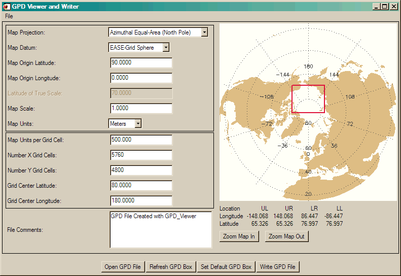
The program I've written is called GPD_Viewer. It is a Catalyst Library program and it requires that both the Coyote and Catalyst Libraries are installed and on your IDL path. You can see a picture of the program in the figure below.
 |
| The GPD_Viewer program. |
The purpose of the program is to be able to see the grid's location, specified by the red box, on the map projection itself. Several map projections (by no means all of them) can be selected from the Map Projection pull-down menu. Several map datums are also available, include WGS84 and other ellipsoid and spherical map datums. The box at the upper left of the window allows you to set map projection information, while the box just below it allows you to specify grid information. One limitation of the program currently is that the only map unit allowed is meters. Clicking on the map projection will center the grid at that location on the map and update the grid values. In this particular case, the grid contains 5760 columns and 4800 rows, with each pixel in the grid representing 500 meters on a side.
If the particular GPD setup shown in the figure was written out, you would have the GPD file shown below.
    ; GPD File Created with GPD_Viewer
   Map Projection:                Azimuthal Equal-Area
   Map Reference Latitude:        90.0000
   Map Reference Longitude:       0.000000
   Map Second Reference Latitude: 70.0000
   Map Scale:                     1.00000
   Map Equatorial Radius:         6370997.00
   Map Polar Radius:              6370997.00
   Map Origin X:                  -1440000.00
   Map Origin Y:                  2310537.95
   Grid Map Units per Cell:       500.000
   Grid Map Origin Column:        -0.5
   Grid Map Origin Row:           -0.5
   Grid Width:                    5760
   Grid Height:                   4800
   ; The following lines are added ONLY to allow easy access to GPD
   ; information by the GPD_Viewer when reading GPD files. Do not remove
   ; them if you wish to read this GPD file in the GPD_Viewer.
   ; GPD Projection:              Azimuthal Equal-Area (North Pole)
   ; Map Datum:                   Sphere
   ; Grid Center Latitude:        80.0000
   ; Grid Center Longitude:       180.000
The keyword/value pairs in the upper part of the GPD file contain the information the NSIDC tools need to project satellite data into this particular map region. The information in the lower part of the file is extra information I need to be able to read GPD files back into the GPD_Viewer. Do not delete this information if you wish to be able to read the GPD file in the GPD_Viewer.
One confusing aspect of GPD files is that the Map Origin X and Y are slightly misnamed. They really represent the origin (or upper left corner) of the grid on the map projection. And, in any case, they use XY (sometimes called UV) map coordinates, rather than the more familiar latitude/longitude coordinates most of us understand. For this reason, the latitude/longitude coordinates of the grid region are also displayed on the GPD_Viewer, underneath the map.
![]()
Using the GPD File to Set Up a Map Coordinate System for an Image
One your satellite data is gridded into a region of the Earth how would you display it using IDL? Suppose you used ms2gt and the GPD file you created above to map MODIS swath data into a Lambert Equal Area projection. Typically these files are saved with a *.img file extension. Suppose this file was named modis_channel_1.img. And suppose the data was scaled between 0 and 1, with most of the values falling between 0.0 and 0.45. You might read it and display the image with these commands. First, to read the data.
    filename = 'modis_channel_1.img'    OPENR, lun, filename, /GET_LUN
   image = FltArr(5760,4800)    ReadU, lun, image    Free_Lun, lun
   image = Reverse(Temporary(image), 2)    sclmin = 0.0    sclmax = 0.45
   imageObj = Obj_New('ScaleImage', image, /NO_COPY, SCLMIN=sclmin, SCLMAX=sclmax, /NOINTERP)
Next, set up a color table for the image and add it to the image object. The "missing" value in this image is 0, so we will make that color white.
   CTLoad, 17, /BREWER, /REVERSE, NCOLORS=254, BOTTOM=1    TVLCT, r, g, b, /GET
   r[0] = 255    g[0] = 255    b[0] = 255    colors = Obj_New('CatColors')
   colors -> SetProperty, COLORPALETTE=[[r],[g],[b]]
   imageObj -> SetProperty, COLOR_OBJECT=colors
Next, we create a map coordinate system for the image, using information we obtain from the GPD file.
   mapCoords = Obj_New('MapCoord', 'Lambert Equal Area', SPHERE_RADIUS=6371228.00, $
       CENTER_LATITUDE=90.0, CENTER_LONGITUDE=0.0)    xorigin = -1440000.0D
   yorigin = 2310578.22D    xend = xorigin + (5760L * 500)
   yend = yorigin - (4800L * 500)    xrange = [xorigin, xend]
   yrange = [yorigin, yend]
   mapCoords -> SetProperty, XRANGE=xrange, YRANGE=yrange
Now we create a map outline a map grid objects, that we add to the map coordinate object, before we pass add all the map objects to the image object.
   outline = Obj_New('Map_Outline', MAP_OBJECT=mapCoords, /HIRES, COLOR='indian red')
   grid = Obj_New('Map_Grid', MAP_OBJECT=mapCoords, COLOR='indian red')
   mapCoords -> SetProperty, OUTLINE_OBJECT=outline, GRID_OBJECT=grid
   imageObj -> SetProperty, COORD_OBJECT=mapCoords
Finally, we display the image in a resizable graphics window.
IMGWIN, imageObj, /WIN_KEEP_ASPECT
You see the result in the figure below. Notice now the MODIS swath data is mapped into the region of the Earth as specified by the GPD file.
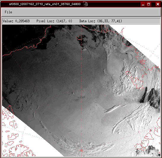 |
| Using the GPD file information to display a gridded MODIS swath image. |
![]()
Version of IDL used to prepare this article: IDL 7.0.3.
![]()
Copyright © 2009 David W. Fanning
Last Updated 5 July 2009