Using the GSHHS Shoreline Database

QUESTION: I find the continental outline database that comes with IDL inadequate sometimes for the kind of detail I need on map projections. Is there an alternative database I can use for more accurate representations of contenental outlines?

ANSWER: You might find the Global Self-consistent, Hierarchical, High-resolution, Shoreline (GSHHS) database more to your liking. The database that comes with IDL is from the World Data Bank (WDB), commonly known as the CIA Data Bank. This data base is quite good for political boundaries, but not as good for shorelines and other land/water boundaries. A very good database for shorelines and land/water boundaries is the World Vector Shoreline (WVS) database. The GSHHS database has been constructed from both the WDB and WVS databases, and is considered to be the best of both databases.

According to the authors, “The data have undergone extensive processing and are free of internal inconsistencies such as erratic points and crossing segments. The shorelines are constructed entirely from hierarchically arranged closed polygons.” The files are released under the GNU Public License.

Perhaps most importantly, the data is available in multiple resolutions, so you can pick the data set most appropriate for your application. The binary files available for downloading are:

gshhs_f.b Full resolution data
gshhs_h.b High resolution data
gshhs_i.b Intermediate resolution data
gshhs_l.b Low resolution data
gshhs_c.b Crude resolution data

Please note that the binary data files are in big-endian byte order. If you are using these data sets on a little-endian machine you will have to flip the byte order. (The usual way to do this is to set the Swap_If_Little_Endian keyword on the READU command).

Reading the Data

You have to be a little bit careful reading the data. Earlier versions of the data used a 40-byte header. Later versions (starting with version 1.6, I believe) used a 32-byte header. However, some versions, for example, gshhs_i.b in version 1.10 used a 32-byte header, but the header was stuffed into a 40 bytes in the data file. Ugh. Version 2.00 of the data base changed the header again. The data I describe in this article uses the 2.2 version of the data. However, I have left various verisons of the header and how you read the header intact in the cgMap_GSHHS program I describe below, so you can select the right version to read the data you happen to have available to you.

The data file is organized and sorted by polygon length (not area) and the locations of each point in the polygon are based on their locations in the full-resolution data set. This is true, even if you are using a lower-resolution data file. Each record, or polygon, in the database contains a 44-byte header (as of version 2.2 of the database) describing the polygon, followed by the X and Y locations of each point in the polygon. (I am using version 2.22 of the GSHHS data, from July 2011, in my example programs.)

Normally, we read each header into a structure variable in IDL defined like this:

   header = { id: 0L, $        ; A unique polygon ID number, starting at 0.
              npoints: 0L, $   ; The number of points in this polygon.
              flag: 0L, $      ; Contains polygon level, version, greenwich, source, and river values.
              west: 0L, $      ; West extent of polygon boundary in micro-degrees.
              east: 0L, $      ; East extent of polygon boundary in micro-degrees.
              south: 0L, $     ; South extent of polygon boundary in micro-degrees.
              north: 0L, $     ; North extent of polygon boundary in micro-degrees.
              area: 0L, $      ; Area of polygon in 1/10 km^2.
              area_full: 0L, $ ; Area of origiinal full-resolution polygon in 1/10 km^2.
              container: 0L, $ ; ID of container polygon that encloses this polygon (-1 if "none").
              ancestor: 0L }   ; ID of ancestor polygon in the full resolution set that was the source
                               ; of this polygon (-1 of "none").

Normally, the binary file is opened for reading with code like this:

   IF N_Elements(filename) EQ 0 THEN BEGIN
      filename = Dialog_Pickfile(Filter='*.b', Title='Select GSHHS File...')
      IF filename EQ "" THEN RETURN
   ENDIF
   OPENR, lun, filename, /Get_Lun, /Swap_If_Little_Endian

Typically, each polygon is read in succession and a decision about whether to draw the polygon or not is made based upon information in the polygon header. For example, you may not want to draw polygons that are smaller than a user-specified minimum area, or you are not interested in ponds inside of islands that inside of lakes, so you can exclude all polygons that have a level of 4. You will probably not be interested in polygons, for example, that are not in the limits of your map projection space. The kind of polygon discrimination you do is entirely up to you. You might use a user-written function to accomplish the descrimination, as shown below. I assume in this code fragment that a map projection has been set up with cgMap_Set prior to this code begin executed, so that the proper latitude/longitude data coordinate system is already established. The user written discrimination function might check to see if the polygon falls within the limits of this map projection space. Sketched roughly, the code will look like this.

   WHILE (EOF(lun) NE 1) DO BEGIN
      READU, lun, header
      
      ; Parse the flag.
      f = header.flag
      version = ISHFT(f, -8) AND 255B
      IF version GT 3 THEN polygonLevel = (f AND 255B) ELSE polygonLevel = header.polygonLevel
      greenwich = ISHFT(f, -16) AND 255B
      source = ISHFT(f, -24) AND 255B

      ; Get the polygon coordinates. Convert to lat/lon.
      polygon = LonArr(2, header.npoints, /NoZero)
      READU, lun, polygon
      lon = Reform(polygon[0,*] * 1.0e-6)
      lat = Reform(polygon[1,*] * 1.0e-6)
      Undefine, polygon

      ; Discriminate polygons based on header information.
      polygonArea = header.area * 0.1
      IF polygonLevel GT level THEN CONTINUE
      IF polygonArea LE minArea THEN CONTINUE

      ; If you have a MAP_PROJECTION structure, use it to warp LAT/LON coordinates.
      ; No point in displaying polygons that are completely outside plot
      ; area set up by a map projection (MAP_SET) or some other plotting command.
      IF N_Elements(map_projection) GT 0 THEN BEGIN
         xy = Map_Proj_Forward(lon, lat, MAP_STRUCTURE=map_projection)
         lon = Reform(xy[0,*])
         lat = Reform(xy[1,*])
      ENDIF

      xy = Convert_Coord(lon, lat, /Data, /To_Normal)
      check = ((xy[0,*] GE !X.Window[0]) AND (xy[0,*] LE !X.Window[1])) AND $
              ((xy[1,*] GE !Y.Window[0]) AND (xy[1,*] LE !Y.Window[1]))
      usePolygon = Max(check)

      IF usePolygon EQ 0 THEN CONTINUE

      ; Draw polygons. Outlines drawn with cgPLOTS, filled polygons drawn with
      ; cgPOLYFILL. Assumes lat/lon data coordinate space is set up.
      IF Keyword_Set(fill) THEN BEGIN
         IF (polygonLevel EQ 1) OR (polygonLevel EQ 3) THEN $
             cgPOLYFILL, lon, lat, Color=land_color, NoClip=0, _EXTRA=extra ELSE $
             cgPOLYFILL, lon, lat, Color=water_color, NoClip=0, _EXTRA=extra
      ENDIF ELSE BEGIN
         cgPLOTS, lon, lat, Color=color, _EXTRA=extra
      ENDELSE

      ; Need outlines with a fill?
      IF Keyword_Set(fill) AND Keyword_Set(outline) THEN $
         cgPLOTS, lon, lat, Color=color, _EXTRA=extra

   ENDWHILE
   Free_Lun, lun

Example Using the GSHHS Database

I have written Coyote Graphics program, named cgMap_GSHHS. The program can be used in a manner similar to Map_Continents. For example, here is code to produce a filled map of Australia.

   datafile = 'gshhs_h.b'
   cgDisplay, 500, 350
   pos = [0.1,0.1, 0.9, 0.8]
   cgMap_Set, -25.0, 135.0, Position=pos, /Mercator, Scale=64e6, Color='black'
   cgColorfill, [pos[0], pos[0], pos[2], pos[2], pos[0]], $
                [pos[1], pos[3], pos[3], pos[1], pos[1]], $
                /Normal, Color='sky blue'
   cgMap_GSHHS, datafile, Fill=1, Level=3, Color='black', /Outline
   cgText, 0.5, 0.85, 'Australia', Font=0, Color='black', /Normal, Alignment=0.5
   cgPlotS, [pos[0], pos[0], pos[2], pos[2], pos[0]], $
            [pos[1], pos[3], pos[3], pos[1], pos[1]], $
            /Normal, Color='black', Thick=2

You see the output of the commands in the figure below.

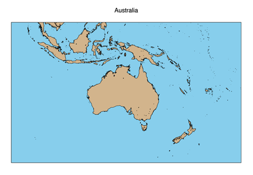Using the GSHHS database with MAP_SET.

The GSHHS dataset can also be used with the map projection structure produced by Map_Proj_Init. Here is an example using a Lambert Azimuthal projection. Notice that cgMap_Continents and cgMap_Grid are used to produce state boundaries and grid lines, features not available in the GSHHS database.

   datafile = 'gshhs_h.b'
   cgDisplay
   map = Obj_New('cgMap', "Lambert Azimuthal", Limit=[40, -95, 50, -75], $
      Center_Lat=45, Center_Lon=-85)
   map -> SetProperty, Position=[0.1, 0.1, 0.90, 0.75], /Draw
   cgMap_GSHHS, datafile, /Fill, Level=3, Map_Structure=map, $
      Water='DODGER BLUE', /Outline, Color='charcoal'
   cgMap_Grid, /Label, /Box, Color='charcoal', Map_Structure=map
   cgText, 0.5, 0.825, 'Great Lakes Region', Font=0, Color='charcoal', $
      /Normal, Alignment=0.5

You see the output of the commands in the figure below.

Using the GSHHS database with MAP_PROJ_INIT via cgMap.