
Overlaying Geographic Data on GeoTIFF Images
QUESTION: I have am trying to display an AVHRR NDVI data image in GeoTIFF format on a map projection in IDL. No matter what I do to georegister the image, the continental outlines are just slightly off. According to the published documentation, this image is in an Albers Conical Equal Area projection, with the corner pixels (from lower-left and in clockwise fashion) located at these latitude/longitude locations:
    longitude =[ -23.490, -24.600, 64.523,  63.414]
   latitude = [ -42.243,  43.711, 43.712, -42.242]
You can see from the image below that the continental outlines I put around the African continent are almost correct, but not exactly correct. The error is especially noticable around Madegascar, but you can see it along the west coast of Africa, as well. Can you help me straighten this out?
 |
| This image is almost registered with the map projection, but not quite. |
![]()
ANSWER: Because this is a GeoTIFF image, the image itself contains information that is suppose to allow the end-user to associate a map projection data coordinate space with the image itself. The data, which is called metadata, is obtained from the GeoTIFF image at the time the image is read into IDL by supplying a GEOTIFF keyword to the READ_TIFF function that reads the image data. A structure, containing GeoTIFF tags is returned by the keyword.
So you can play along if you like, I have made a GeoTIFF image available to you on my web page. Extract the GeoTIFF image to the same directory in which you will run the example IDL code, which I have named tiffoverlay.pro.
To open the GeoTIFF file and read it into IDL, type these commands.
    filename = 'AF03sep15b.n16-VIg.tif'
   image = Read_Tiff(filename, GEOTIFF=geotag)    image = Reverse(image, 2)
Notice we have collected the GeoTIFF metadata into an IDL structure variable named geotag, and that we have reversed the Y direction of the image. The latter is almost always required when working with TIFF images in IDL, since the TIFF standard sets the (0,0) point in the upper-left corner of the image, and IDL almost always prefers to use the lower-left corner of the image for that purpose. I always reverse the actual image data, rather than just display the image "upside down" by setting the !Order system variable, since I often want to interact with images, and I want to avoid the confusion that is inevitable when my “location in the image” is different from my “display of the image” in the graphics window.
The GeoTIFF meta data is available as geotags, which are represented in IDL as fields in the geotag structure.
    IDL> Help, geotag, /Structure
  ** Structure, 17 tags, length=144, data length=138, refs=1:
     MODELPIXELSCALETAG      DOUBLE    Array[3]
     MODELTIEPOINTTAG        DOUBLE    Array[6, 1]
     GTMODELTYPEGEOKEY       INT              1
     GTRASTERTYPEGEOKEY      INT              1
     GEOGRAPHICTYPEGEOKEY    INT           4326
     GEOGLINEARUNITSGEOKEY   INT           9001
     GEOGANGULARUNITSGEOKEY  INT           9102
     PROJECTEDCSTYPEGEOKEY   INT          32767
     PROJECTIONGEOKEY        INT          32767
     PROJCOORDTRANSGEOKEY    INT             11
     PROJLINEARUNITSGEOKEY   INT           9001
     PROJSTDPARALLEL1GEOKEY  DOUBLE          -19.000000
     PROJSTDPARALLEL2GEOKEY  DOUBLE           21.000000
     PROJNATORIGINLONGGEOKEY DOUBLE           20.000000
     PROJNATORIGINLATGEOKEY  DOUBLE           1.0000000
     PROJFALSEEASTINGGEOKEY  DOUBLE          0.00000000
     PROJFALSENORTHINGGEOKEY DOUBLE          0.00000000
Unfortunately, most of this information doesn't mean much to you, probably, and the IDL documentation doesn't help you sort it out. To understand it, you are probably going to have to go to somewhere like RemoteSensing.org, where you can find documentation on the GeoTIFF format itself. The piece of software I have found most helpful in understanding GeoTIFF files is listgeo, which provides a dump of the GeoTIFF metadata in a human readable form. On my Windows machines, I use a GUI wrapper to listgeo, named listgeo_GUI. It is not elegant software, but I do find it essential.
To understand the specific geotags you find in your GeoTIFF file, you are going to have to search through the GeoTIFF file specifications. I usually search for the specific geotag name in this document. The information I need is typically found in the Appendices of this document.
Here is a slightly edited portion of the listgeo printout for this file. It will help you see how you can find the same information in the GeoTIFF tags directly from within IDL.
    Geotiff_Information:       Version: 1       Key_Revision: 1.0
      Tagged_Information:          ModelTiepointTag (2,3):
            0                0                0
            -4599918.34      4600147.47       0
         ModelPixelScaleTag (1,3):
            8000             8000             0
         End_Of_Tags.     Projection Method: CT_AlbersEqualArea
      ProjStdParallel1GeoKey: -19.000000 ( 19d 0' 0.00"S)
      ProjStdParallel2GeoKey: 21.000000 ( 21d 0' 0.00"N)
      ProjNatOriginLatGeoKey: 1.000000 (  1d 0' 0.00"N)
      ProjNatOriginLongGeoKey: 20.000000 ( 20d 0' 0.00"E)
      ProjFalseEastingGeoKey: 0.000000 m
      ProjFalseNorthingGeoKey: 0.000000 m    GCS: 4326/WGS 84
   Datum: 6326/World Geodetic System 1984
   Ellipsoid: 7030/WGS 84 (6378137.00,6356752.31)
   Prime Meridian: 8901/Greenwich (0.000000/  0d 0' 0.00"E)
   Projection Linear Units: 9001/metre (1.000000m)     Corner Coordinates:
   Upper Left    (-4599918.340, 4600147.470)
   Lower Left    (-4599918.340,-4615852.530)
   Upper Right   ( 4616081.660, 4600147.470)
   Lower Right   ( 4616081.660,-4615852.530)
   Center        (    8081.660,   -7852.530)
We see that the image is in an Albers Equal Area map projection. (We can obtain this information from the metadata by translating the PROJECTIONGEOKEY and PROJCOORDTRANSGEOKEY geotags--or fields in the geotag structure--according to the information in the GeoTIFF specifications.) Other information essential for setting up the map projection is also avaiable. For example, the Albers Equal Area projection requires two standard parallels and these are provided in the PROJSTDPARALLEL1GEOKEY and PROJSTDPARALLEL2GEOKEY geotags. The datum used for this projection is WGS84 (a translation of the GEOGRAPHICTYPEGEOKEY geotag, 4326). We can find the center of the map projection in the PROJNATORIGINLATGEOKEY and PROJNATORIGINLONGGEOKEY geotags.
In addition to knowing what particular map projection was used for the image, we have to know where, exactly, the image is located in that map projection. This information is also available in the geotags, but you have to know how to parse it. Of particular importance are the tie points (MODELTIEPOINTTAG) and the image scale (MODELPIXELSCALETAG). The tie points usually (but not always) locate the upper left corner of the image in Cartesian coordinates. This is simply a flat 2D surface upon which we cast the map projection and upon which we draw a grid in arbitrary units. In this case, the units are meters (from the PROJLINEARUNITSGEOKEY tag) and the extent of the grid is the diameter of the Earth. This arbitrary coordinate system is sometimes called the UV coordinate system, where U is the X dimension (often associated with longitude) and V is the Y dimension (often associated with latitude).
It is in this coordinate system that the corners and center of the image are reported in the listgeo information above. But we can calculate the corner values ourselves from within IDL. Here is the code to do it. In this code, you will see that I have moved the origin of the image from the upper-left to the lower-left. This is not strictly necessary, but I do it for my own sanity. I have been working with IDL so long that I just assume the origin is at the lower-left and I make too many mistakes if it is not. The end points are found by using the tie-points as the starting coordinates and then just multipling the size of the image in each dimension by the scaling factor for that dimension.
   ; Find the image dimensions.    s = Size(image, /Dimensions)
    ; Calculate corner points from GeoTIFF structure obtained from file.
   xscale  = geotag.ModelPixelScaleTag[0]
   yscale  = geotag.ModelPixelScaleTag[1]
   tp      = geotag.ModelTiePointTag[3:4]
   ; Origin in upper-left in TIFF file. I want to move to bottom left
   ; for my own sanity.    xOrigin = tp[0]    yOrigin = tp[1] - (yscale * s[1])
   xEnd = xOrigin + (xscale * s[0])    yEnd = tp[1]
   ; Print the corner coordinates. They correspond exactly to what is in TIFF file
   ; according to listgeo from www.remotesensing.org.
   Print, 'Corner Coordinates:'
   Print, 'Upper Left:  (' + String(xOrigin, Format='(D0.3)') + $
          ', ' + String(yEnd, Format='(D0.3)') + ')'
   Print, 'Lower Left:  (' + String(xOrigin, Format='(D0.3)') + $
          ', ' + String(yOrigin, Format='(D0.3)') + ')'
   Print, 'Upper Right: (' + String(xEnd, Format='(D0.3)') + ', ' + $
           String(yEnd, Format='(D0.3)') + ')'
   Print, 'Lower Right: (' + String(xEnd, Format='(D0.3)') + ', ' + $
           String(yOrigin, Format='(D0.3)') + ')'
You can see from the print-out, that this calculation is identical to the corners reported by listgeo.
    Corner Coordinates:
   Upper Left:  (-4599918.340,  4600147.470)
   Lower Left:  (-4599918.340, -4615852.530)
   Upper Right: ( 4616081.660,  4600147.470)
   Lower Right: ( 4616081.660, -4615852.530)
The next step is to find out where the corners of the image are in latitude and longitude space, rather than UV space. To put our image into the UV space we had to transform the data via a map projection. (In other words, our image represented some portion of a 3D surface, and we transformed that, via a map projection, into the 2D surface of the UV coordinate system.) To get back into a 3D coordinate system, represented by latitude and longitude coordinates, we have to perform an inverse transformation. We do so with MAP_PROJ_INVERSE, but to use it we have to establish the map projection space with MAP_PROJ_INIT. The code looks like this. (I have ordered the arguments so the coordinates start in the lower-left corner of the image and proceed clockwise, so the values can be compared with the published corner values.)
    ; Map the corners in lat/lon space by inverse transformation.
    alberMap = MAP_PROJ_INIT('Albers Equal Area Conic', $
       DATUM=8, $ ; WGS84        CENTER_LAT=geotag.PROJNATORIGINLATGEOKEY, $
       CENTER_LON=geotag.PROJNATORIGINLONGGEOKEY, $
       STANDARD_PAR1=geotag.PROJSTDPARALLEL1GEOKEY, $
       STANDARD_PAR2=geotag.PROJSTDPARALLEL2GEOKEY)
    lonlat = MAP_PROJ_INVERSE([xOrigin, xOrigin, xEnd, xEnd], $
                              [yOrigin, yEnd, yEnd, yOrigin], $
                               MAP_STRUCTURE=alberMap)
Printing these latitude/longitude values out, you can see they are not the same as the published values. Having spent a fair amount of time working with satellite image documentation, I would not be surprised to find the published results just simply wrong. It happens all the time. But, I think in this case, the published results describe the locations of the center of the corner pixels, and in IDL we need to work with the pixel edges. So, if you wanted to use the published corner values, you would have to move their locations by half a pixel in both the U and V dimensions to get an accurate map overlay.
    Published Values:    longitude = [ -23.490, -24.600, 64.523,  63.414]
   latitude =  [ -42.243,  43.711, 43.712, -42.242]      Calculated Values:
   longitude = [-23.477562, -24.589251, 64.745913,  63.630319]
   latitude =  [-42.209247,  43.416786, 43.414412, -42.211575]
To overlay data on the map projection, the extent of the map projection has to be exactly coincident with the image. Thus, we have to know the limits of the map projection. We can try to calculate those from the corner pixels. Choosing two opposite corners that have the maximum separation, we write code like this.
   ; The limit is the min and max of these latitudes and longitudes.
   minLat = Min(lonlat[1,*], MAX=maxLat)
   minLon = Min(lonlat[0,*], MAX=maxLon)
   limit = [minLat, minLon, maxLat, maxLon]
Unfortunately, you can see (from the calcuated longitude and latitude values above) that the limit doesn't exactly describe the location of the image on the map. We really need an eight-element limit array to describe the four corners of the image. Something like that exists in IDL for the MAP_SET command. (Although you must specify the left, top, right, and bottom location of the image, and not the corners.) But if we pass an eight-element array to the LIMIT keyword in MAP_PROJ_INIT it doesn't complain, but it completely ignores the values!
Let's see what happens if we continue to use the limit as we calculate above.We use MAP_PROJ_INIT, but with the LIMIT keyword set.
   ; Set up a map projection space, using a limit.
   alberMap = MAP_PROJ_INIT('Albers Equal Area Conic', $
      DATUM=8, $ ; WGS84       CENTER_LAT=geotag.PROJNATORIGINLATGEOKEY, $
      CENTER_LON=geotag.PROJNATORIGINLONGGEOKEY, $
      STANDARD_PAR1=geotag.PROJSTDPARALLEL1GEOKEY, $
      STANDARD_PAR2=geotag.PROJSTDPARALLEL2GEOKEY, $       LIMIT=limit)
The MAP_PROJ_INIT function returns a map structure variable. One of the fields in this structure variable is UV_BOX. This field describes the extent of the map in UV coordinates. You will have to use this UV_BOX to set up a data coordinate system that you can draw on top of with MAP_CONTINENTS and MAP_GRID.
First, we set up the display and display the image. You will need programs from the Coyote Library if you wish to execute this part of the code.
   ; Erase the display and set up an image position.
   IF (!D.Flags AND 256) NE 0 THEN cgErase, 'ivory'    pos = [0,0,1,1.]
   ; Set up color table.    cgLoadCT, 0    TVLCT, cgColor('ivory', /Triple), 0
   cgLoadCT, 33, NColors=253, Bottom=1     ; Scale the image.
   scaled = BytScl(image, Top=253)+1    index = Where(scaled EQ 1)
   scaled[index] = 0B     ; Display the image.
   cgDisplay, 500, 500, WID=0, Title='Outline using UV_BOX with Incorrect Limits.', $
      XPOS=10, YPOS=10    cgImage, scaled, POSITION=pos, /KEEP_ASPECT
Next we set up the UV data coordinate system. This is where we use the UV_BOX of the map structure. Notice the PLOT command is constructed in such a way that nothing is actually drawn on the display. Its purpose is simply to set the appropriate system variables that will establish the UV data coordinate system.
   ; Use the (slight wrong) UV_BOX of map structure to set up the data coordinate space.
   uv_box = alberMap.uv_box    Print, 'MAP_PROJ_INIT UV_BOX:  ', uv_box
   cgPlot, uv_box[[0, 2]], uv_box[[1, 3]], Position=pos, $
          /Nodata, XStyle=5, YStyle=5, /NoErase
Finally, we can draw political boundaries and grid lines. Note that we have to pass the map structure to MAP_CONTINENTS and MAP_GRID so they have the means to convert their latitude/longitude data into the proper UV coordinates.
    ; Draw political boundaries and coasts.
    cgMap_Continents, /HIRES, Color='Dark Slate Blue', $
	   Map_Structure=alberMap, /COUNTRIES, /COASTS      ; Add gridlines
    cgMap_Grid, /LABEL, Color='Slate Blue', Map_Structure=alberMap
You see the result in the figure below. Notice that the boundaries are just ever so slightly off. You will notice this particularly around Madagascar, in the lower-right corner of the figure.
 |
|
| The overlays don't quite match up. This is because we weren't able to specify the location of the image in the map projection exactly. This is a limitation of the LIMIT keyword of MAP_PROJ_INIT. It needs to be able to accept an eight-element LIMIT keyword instead of just a four-element LIMIT keyword. | |
Just for completeness, let's calculate an eight-element LIMIT keyword, as we could do if we were specifying the lat/lon data coordinate space with a MAP_SET command. The code would look like this, in which I am calculating the left, top, right, and bottom sides of the image.
    lonlat = MAP_PROJ_INVERSE([xOrigin, xOrigin, xEnd, xEnd   ], $
                              [yOrigin, yEnd,    yEnd, yOrigin], $
                               MAP_STRUCTURE=alberMap)
    lefty =  Abs(lonlat[1,0]-lonlat[1,1])/2.0 + Min([lonlat[1,0],lonlat[1,1]])
    leftx =  Abs(lonlat[0,0]-lonlat[0,1])/2.0 + Min([lonlat[0,0],lonlat[0,1]])
    topy =   Abs(lonlat[1,1]-lonlat[1,2])/2.0 + Min([lonlat[1,1],lonlat[1,2]])
    topx =   Abs(lonlat[0,1]-lonlat[0,2])/2.0 + Min([lonlat[0,1],lonlat[0,2]])
    righty = Abs(lonlat[1,2]-lonlat[1,3])/2.0 + Min([lonlat[1,2],lonlat[1,3]])
    rightx = Abs(lonlat[0,2]-lonlat[0,3])/2.0 + Min([lonlat[0,2],lonlat[0,3]])
    boty =   Abs(lonlat[1,3]-lonlat[1,0])/2.0 + Min([lonlat[1,3],lonlat[1,0]])
    botx =   Abs(lonlat[0,3]-lonlat[0,0])/2.0 + Min([lonlat[0,3],lonlat[0,0]])
    limit = [lefty, leftx, topy, topx, righty, rightx, boty, botx]
    alberMap = MAP_PROJ_INIT('Albers Equal Area Conic', $
      DATUM=8, $ ; WGS84       CENTER_LAT=geotag.PROJNATORIGINLATGEOKEY, $
      CENTER_LON=geotag.PROJNATORIGINLONGGEOKEY, $
      STANDARD_PAR1=geotag.PROJSTDPARALLEL1GEOKEY, $
      STANDARD_PAR2=geotag.PROJSTDPARALLEL2GEOKEY, $       LIMIT=limit)
   cgDisplay, 500, 500, WID=1, Title='Attempt Using Correct 8-Element Limits', $
      XPOS=10, YPOS=10    cgImage, scaled, POSITION=pos, /KEEP_ASPECT
   ; We use the UV_BOX returned from MAP_PROJ_INIT with eight-element LIMIT.
   uv_box = alberMap.uv_box    Print, '8-Element UV_BOX:      ', uv_box
   cgPlot, uv_box[[0, 2]], uv_box[[1, 3]], Position=pos, $
          /Nodata, XStyle=5, YStyle=5, /NoErase
    ; Draw political boundaries and coasts.
    cgMap_Continents, /HIRES, Color='Dark Slate Blue', $
	   Map_Structure=alberMap, /COUNTRIES, /COASTS      ; Add gridlines
    cgMap_Grid, /LABEL, Color='Slate Blue', Map_Structure=alberMap
You can see in the results below that the MAP_PROJ_INIT command takes the eight-element LIMIT, but ignores its values.
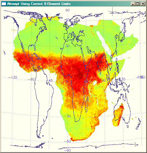 |
|
| The MAP_PROJ_INIT command takes an eight-element LIMIT, but completely ignores its values. The UV_BOX produced is completely wrong. | |
To reiterate, the problem is that we cannot extract the exact limit of the map projection for this image with a four-element LIMIT array. But, in fact, we already have the proper limits calculated from before. These are the coordinates that we put into variables xOrigin, xEnd, yOrigin, and yEnd. We simply use these variables to set up our data coordinate space. The code looks like this.
   cgDisplay, 500, 500, WID=1, Title='Outline using Correct Calculated Limits.', $
      XPOS=20, YPOS=20    cgImage, scaled, POSITION=pos, /KEEP_ASPECT
   ; Use the calculated UV_BOX to set up the data coordinate space.
   uv_box = [xOrigin, yOrigin, xEnd, yEnd]
   Print, 'Calculated UV_BOX:     ', uv_box
   cgPlot, uv_box[[0, 2]], uv_box[[1, 3]], Position=pos, $
          /Nodata, XStyle=5, YStyle=5, /NoErase
   ; Draw political boundaries and coasts.
   cgMap_Continents, /HIRES, Color='Dark Slate Blue', $
	   Map_Structure=alberMap, /COUNTRIES, /COASTS     ; Add gridlines
   cgMap_Grid, /LABEL, Color='Slate Blue', Map_Structure=alberMap
You see the correct results in the figure below.
 |
|
| This image uses the calculated limits from the GeoTiff file to set up the data coordinate space and the result is perfect. | |
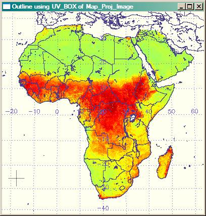
An alternative way to get perfect results, is to use the UV_BOX from MAP_PROJ_IMAGE via its UVRANGE keyword, rather than from the MAP_PROJ_INIT map structure. (After a great deal of effort, I learned this is how iMap manages to get the outlines around its maps perfect.) The MAP_PROJ_IMAGE command, unlike the MAP_PROJ_INIT command, does use an eight-element positioning keyword to calculate the UV_BOX. The commands are similar to those above. And the result looks identical to the figure directly above.
   cgDisplay, 500, 500, WID=3, Title='Outline using UV_BOX of Map_Proj_Image', $
      XPOS=30, YPOS=30    cgImage, scaled, POSITION=pos, /KEEP_ASPECT
   ; Use the UV_BOX of Map_Proj_Image to set up the data coordinate space.
   warp = Map_Proj_Image(dist(10), $
      [xorigin, yorigin, xend, yend], $ ; image range in UV coords
      Image_Structure=alberMap, $       Map_Structure=alberMap, $
      UVRANGE=uv_box)        Print, 'MAP_PROJ_IMAGE UV_BOX: ', uv_box
   cgPlot, uv_box[[0, 2]], uv_box[[1, 3]], Position=pos, $
          /Nodata, XStyle=5, YStyle=5, /NoErase
   ; Draw political boundaries and coasts.
   cgMap_Continents, /HIRES, Color='Dark Slate Blue', $
	   Map_Structure=alberMap, /COUNTRIES, /COASTS     ; Add gridlines
   cgMap_Grid, /LABEL, Color='Slate Blue', Map_Structure=alberMap
The UV_BOX values for the four methods are shown below. Notice that the UV_BOX coordinates are identical for the last two methods.
   MAP_PROJ_INIT UV_BOX:        -4717397.8      -4644644.7       4733971.2       4600353.9
   8-Element UV_BOX:            -19170318.      -6842903.5       18106165.       7207980.3
   Calculated UV_BOX:           -4599918.3      -4615852.5       4616081.7       4600147.5
   MAP_PROJ_IMAGE UV_BOX:       -4599918.3      -4615852.5       4616081.7       4600147.5
Many thanks to Matt Savoie for his help in solving this long standing mystery.
![]()
Coyote Graphics Map Object
The Coyote Graphics program cgGeoMap can do all of this georegistration for you and create a map object (cgMap) that can set up the map data coordinate system for you automatically. It can even read and return the image to you from the TIFF file. The commands to do so will look like this.
    filename = 'AF03sep15b.n16-VIg.tif'
   cgDisplay, 500, 500, WID=5, Title='Outline cgMap Object', $
      XPOS=50, YPOS=50
   alberMap = cgGeoMap(filename, IMAGE=tiffImage, /OnImage)
   scaled = BytScl(tiffImage, Top=253)+1    index = Where(scaled EQ 1)
   scaled[index] = 0B    TVLCT, cgColor('ivory', /Triple), 0
   cgLoadCT, 33, NColors=253, Bottom=1
   cgImage, scaled, POSITION=pos, /KEEP_ASPECT
   ; Set up a map coordinate system.    alberMap -> Draw
   ; Draw political boundaries and coasts.
   cgMap_Continents, /HIRES, Color='Dark Slate Blue', $
	   Map_Structure=alberMap, /COUNTRIES, /COASTS     ; Add gridlines
   cgMap_Grid, /LABEL, Color='Slate Blue', Map_Structure=alberMap
![]()
Version of IDL used to prepare this article: IDL 7.1.
![]()
Copyright © 2008 David W. Fanning
Written 14 March 2008
Last Updated 22 November 2011