Gridding XYZ Triples to Form a Surface Plot

QUESTION: I have some surface data that is generated by an external program as XYZ values. Can I display this data as a surface in IDL?

ANSWER: Yes you can, but not without some manipulation. All the surface-generating commands in IDL (e.g., SURFACE, IDLgrSURFACE) require that the surface data be expressed as a 2D array of values. The easiest way to create such a 2D array from your XYZ data is to grid the data using the IDL commands TRIANGULATE and TRIGRID. Here is how that works. (You can download the sample code and run the program yourself, if you like.)

First, let's create some XYZ data that will represent the surface we want to display. The X and Y data points are randomuly distributed in space. The Z data points depends upon X and Y. It is the Z data that we want to visualize as a surface.

   seed = -1L
   x = RandomU(seed, 41)
   y = RandomU(seed, 41)
   z = Exp(-3*((x - 0.5)^2 + (y - 0.5)^2))

Here is the random distribution of XY points in space.

    cgDisplay, WID=1, Title='XY Point Distribution', $
       400, 350, XPos=0, YPos=0
    cgPlot, Findgen(41), /NoData, $
       XRange=[0, Max(x)], YRange=[0, Max(y)]
    cgPlotS, x, y, PSym=1, Color='red'

You see the results of these commands in this graphic illustration.

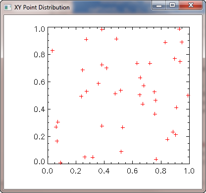Random distribution of XY points in space.

 

The next step in the gridding process is to create a set of Delaunay triangles from the XY points, using the TRIANGULATE command. We pass in the X and Y data vectors and get a set of triangles returned. In this case, we are also going to return an optional set of boundary points that can be used to extrapolate the surface outside the actual set of points in the XY vectors. Extrapolation sometimes this gives a smoother looking surface when we visualize it.

   Triangulate, x, y, triangles, boundaryPts

It is useful sometimes to see the set of triangles that is produced, as it gives you some insight into how the 2D surface array will be created. To visualize the triangles, type this:

    s = Size(triangles, /Dimensions)
    num_triangles = s[1]
    cgDisplay, WID=2, Title='Delanay Triangles', $
       400, 350, XPos=415, YPos=0
    cgPlot, Findgen(41), /NoData, $
       XRange=[0, Max(x)], YRange=[0, Max(y)]
    
    ; Draw the triangles.
    FOR j=0,num_triangles-1 DO BEGIN
        thisTriangle = [triangles[*,j], triangles[0,j]]
        cgPlotS, x[thisTriangle], y[thisTriangle], Color='teal'
    ENDFOR
    
    ; Overplot the points.
    cgPlotS, x, y, PSym=1, Color='red'

You see the results of these commands in this graphic illustration.

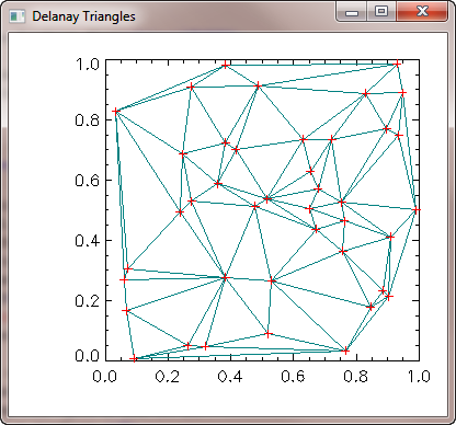The Delaunay triangles produced by TRIANGULATE.

 

The next step is to create the gridded 2D array from these Delaunay triangles. What will happen is that IDL will use the values at each triangle vertex to interpolate intermediate values along a regular grid.

Although it is not required here (TRIGRID can figure it out on its own), it is sometimes a good idea to decide what kind of grid spacing you would like in your output 2D array. Let's suppose we want to sample this data at intervals of 0.01 units in X and 0.05 units in Y. We could set up our grid spacing vector like this:

   gridSpace = [0.01, 0.05]

We use the TRIGRID command to created the 2D gridded array, like this. (The XGRID and YGRID keywords are used to return X and Y vectors that can be used with the 2D gridded array in the cgSurf command to come.)

   griddedData = TriGrid(x, y, z, triangles, gridSpace, $
      XGrid=xvector, YGrid=yvector)

To visualize the 2D gridded array, we use the cgSurf command. Notice that you can make out some of the faces of the triangles in this initial surface plot. In other words, the gridding is not done very smoothly.

   cgSurf, griddedData, xvector, yvector, XStyle=1, YStyle=1

You see the results of these commands in this graphic illustration.

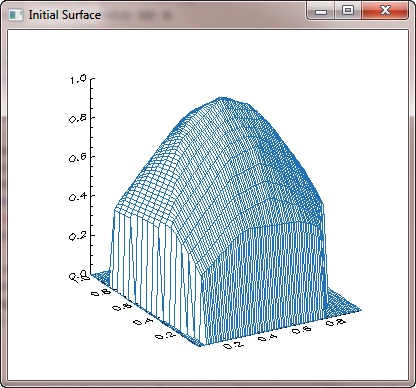The initial gridded surface.

 

To create a smoother surface, you can set the Quintic keyword on the TRIGRID command. This will cause IDL to use a quintic polynomial fit in the interpolation of the data points, resulting in a much smoother surface.

   griddedData = TriGrid(x, y, z, triangles, gridSpace, $
      XGrid=xvector, YGrid=yvector, /Quintic)
  cgSurf, griddedData, xvector, yvector, XStyle=1, YStyle=1

You see the results of these commands in this graphic illustration.

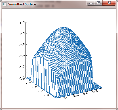The smoothed gridded surface.

 

Finally, you notice that we have created a surface that is totally within the bounds of the initial X and Y vectors. But it might be more realistic to extrapolate the surface in the range of the potential data, rather than in the range of the actual data. The potential data range in this case is 0 to 1 in X and Y, although neither the X or Y vector has values at these extremes.

We can use the boundary points that were returned to us in the TRIANGULATE command to extrapolate outside the actual data. You don't always want to do this, but in this case I think it makes a better surface plot. You pass the boundary points to the TRIGRID command, like this.

   griddedData = TriGrid(x, y, z, triangles, gridSpace, $
      XGrid=xvector, YGrid=yvector, /Quintic, Extrapolate=boundaryPts)
  cgSurf, griddedData, xvector, yvector, XStyle=1, YStyle=1

You see the results of these commands in this graphic illustration.

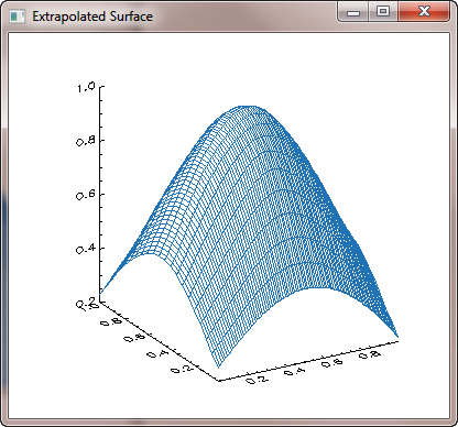The quintic smoothed gridded surface.

 

[Return to IDL Programming Tips]