
Improved Image Contrast
QUESTION: I have an image, but it has very low contrast. How can I improve the contrast in this image so I can see more of the image detail?
![]()
ANSWER: Image contrast falls under the general category of image pixel transformations. If you are interested in learning more, I wholeheartedly recommend Digital Image Processing, 2nd Edition, by Gonzalez and Woods. And if you are trying to write IDL code from what you learn, I recommend their companion volume, Digital Image Processing Using MATLAB. Both are excellent resources. Chapter 3 of both books is devoted to this topic.
Linear Contrast Scaling
The standard IDL routine for providing image contrast is BytScl. The input 2D image is scaled into full color dynamic range of 0 to 255 with a linear scaling function. [Note that programs from the Coyote Library are required to work the following IDL examples.]
   IDL> knee= SelectImage(/Examples, Filename="mr_knee.dcm", /FlipImage)
   IDL> cgMinMax, knee
        1024    1284
   IDL> scaledImage = BytScl(knee)
   IDL> cgMinMax, scaledImage
        0    255
While a linear scaling enables you to see an image on your display that you couldn't see otherwise (image pixels have to be scaled into the range 0 to 255 to be seen), it does little to improve image contrast. To improve contrast, you typically choose a minimum and maximum threshold value and scale the data linearly between those two values.
For example, the image below on the left is displayed with just the BytScl command, like this.
IDL> cgImage, BytScl(knee)
Whereas the image on the right uses a minimum threshold value of 1080 and a maximum threshold value of 1200.
IDL> cgImage, BytScl(knee, MIN=1080, MAX=1200)
When thresholding, all values in the image below the minimum threshold value are set to the threshold value before linear scaling occurs. Similarly, all values in the image greater than the maximum threshold value are set to the maximum threshold value before scaling. Notice the difference in contrast in the resulting image.
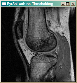 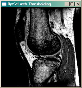 |
| The image on the left is byte scaled. The image on the right is byte scaled with a minumum threshold of 1080 and a maximum threshold of 1200. |
The difference between the minimum and maximum threshold values is often called the “window”, and the center of the window is called the “level”. In medical images, especially, we often write applications that allow us to change the size of the window, and the window level interactively. This is called “windowing and leveling.”
In contrast enhancement, the threshold values are selected to emphasize features of interest. Typically, the image histogram provides one empirical method for rational threshold selection. Consider, for example, the CTSCAN data set provided with IDL.
   IDL> scan = cgDemoData(5)
   IDL> scan = Reverse(Temporary(scan), 2)
If we look at a histrogram of the image pixels, next to the byte scaled image itself, we see that most of the image pixels are confined to the pixel range 50 to 100. The image itself is of low contrast.
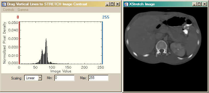 |
| The image histogram on the left and the image on the right. Most of the image pixels fall into a narrow dynamic range between 50 and 100. |
If we set the minimum threshold at 50 and the maximum threshold at 100, then we are able to improve the image contrast and see more detail in the image. Consider the figure below.
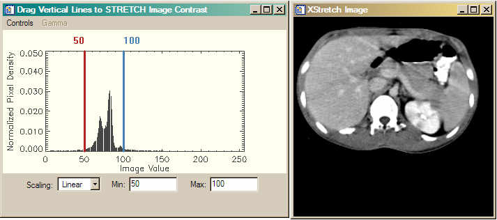 |
| Here the threshold values are choosen so that the linear stretch is applied to the vast majority of information containing pixels in the image. Note the difference in appearance of the stretched image. |
Interactive Scaling with cgSTRETCH
The cgStretch command is providing the image histogram in the figures above. cgStretch is a graphical and interactive front end for the four different kinds of image scaling we will be discussing in this article. The threshold lines (shown in red and blue colors) can be interactively moved by the user to get immediate feedback on how the changes affect the image.
IDL> cgStretch, scan
The cgStretch program can save the scaled image to the main IDL level for future processing, etc. Moveover, the image and histogram windows can be saved directly to JPEG, TIFF, PNG, PostScript and other types of files to preserve a record of your session. Formatted 2D image files (JPEG, TIFF, PNG, FITS, DICOM, etc.) can be read directly into the program (through the use of SelectImage). Both the histogram and the image window are resizeable. The image window will only resize to a size that preserves the aspect ratio of the image.
![]()
Power-Law or Gamma Scaling
While linear scaling is useful for many images, and especially for those images collected under ideal conditions, it is often less useful for images collected under more difficult conditions. Such images often have low signal to noise ratios, small dynamic ranges, or other problems that result in low contrast images. Astronomical and medical images often fall into this category. In this case, some kind of logarithmic scaling is usually needed for improved image contrast.
There are two types of logarithmic scaling in common use. One uses a power law scaling. This is typically known as “gamma” scaling. And the other uses a more typical logarithmic scaling factor. Let's first consider gamma scaling.
In gamma scaling, the input image is raised to a gamma power, like this:
scaledImage = image^gamma
Gamma values typically range from 0.04 to 25.0. A gamma value of 1.0 is a linear scaling. Gamma values less than 1.0 map darker image values into a wider range of output values, while a gamma value greater than 1.0 maps lighter image values into a wider range of output values. The figure below shows typical scaling curves for various gamma values.
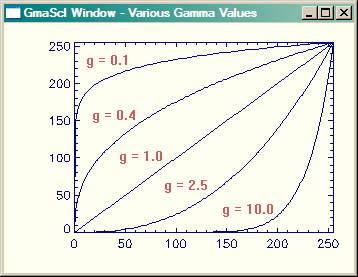 |
| Scaling curves for various values of gamma. Input values are along the X axis and output values are along the Y axis |
Gamma scaling is slightly more difficult to do than linear scaling, so I have written a program to do it for me. The program is named GmaScl. I think of it as BytScl on steroids, because it can do the same kind of linear scaling BytScl does, but it does it in a more convenient way. And, of course, it also allows you to specify a gamma factor for a power-law scaling function. For example, we can apply a gamma scaling to the CT scan data set, like this.
IDL> cgImage, GmaScl(scan, GAMMA=2.5, MIN=50, MAX=100)
Or, we can use cgStretch do to the same thing interactively. Simply choose “Gamma” from the list of scaling options, and select a desired gamma factor from the Gamma pull-down menu in the menubar. A third line (drawn in green in this example) is drawn on the image histogram to give you a sense of how the function is being applied to the data. In the example below, you see that with a gamma factor of 2.5, and with thresholding at 50 and 100, we are emphasising the pixel values between about 75 and 100.
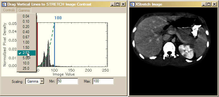 |
| A gamma scale factor of 2.5 is applied to the CT scan data set. Note that the function is drawn on the image histogram to give you a sense of which pixels are being emphasized by the gamma scaling. |
Restricting the Output Data Range
Sometimes you do not want the output data range to extend from 0 to 255. For example, you might want the data range to be between 50 and 200. With BytScl you would have to do something like this
   IDL> cgMinMax, BytScl(scan, TOP=150, MIN=35, MAX=105) + 50B
        50   200
With GmaScl (and with LogScl and AsinhScl, described below), you can use the keywords OMIN and OMAX to do the same thing.
   IDL> cgMinMax, GmaScl(scan, OMIN=50, OMAX=200, MIN=35, MAX=105, GAMMA=2.5)
        50   200
![]()
Log Scaling
Another common scaling function is a logarithmic function. The one I use is this:
scaledImage = 1 / ( 1 + (mean/image)^exponent)
Where mean is a value between 0 and 1 that positions the center of the log curve with respect to the threshold values. A mean value of 0.5 centers the curve between the threshold values. The variable exponent is similar to the gamma factor.
A log scaling curve like this tends to compress the image values near the threshold values, and to linearly scale the values between the tails of the curve. By adjusting the exponent value, you can increase or decrease the slope of the linear portion of the curve. I have written the program LogScl to implement this scaling factor.
IDL> cgImage, LogScl(scan, MIN=35, MAX=115, MEAN=0.5, EXPONENT=8)
Or, we can use cgStretch do to the same thing interactively. Simply choose “Log” from the list of scaling options, and type in your desired mean and exponent values in the input fields. A third line (drawn in green in this example) is drawn on the image histogram to give you a sense of how the function is being applied to the data. In the example below, you see that with a mean of 0.5, and and exponent of 8, we get a fairly steep linear portion of the curve centered between 35 and 115.
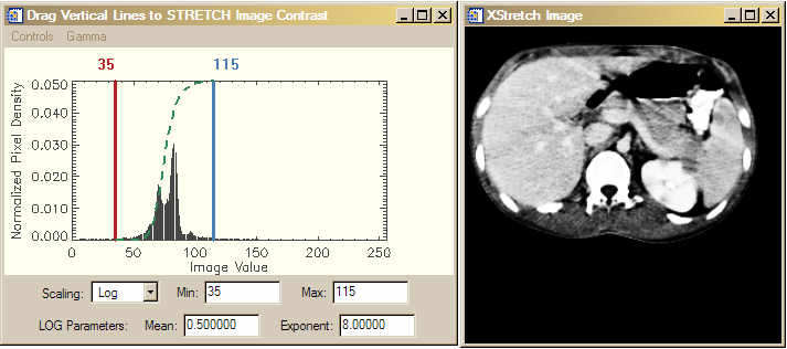 |
| A logarithmic scaling function applied to the image. |
![]()
Inverse Hyperbolic Sine Scaling
A fourth type of image contrast scaling that is particularly common with astronomical images uses an inverse hyperbolic sine function to perform the scaling. This function produces a scaling curve with a linear section, which is usually used to model noise in the image, and a logarithmic section which is used to model image flux values, which can often vary by orders of magnitude. The curve is tuned or softened by means of a BETA keyword. Smaller values of BETA make the linear portion of the curve short and steep, whereas larger values of BETA make the linear portion of the curve longer and flatter. This function is particularly effective with low-flux astronomical images.
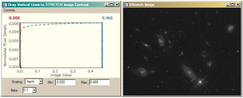 |
| An inverse hyperbolic sine scaling function is applied to this low-flux astronomical image. This function gave the best results of all the scaling functions for this astronomical image. |
All of these stretches and more (e.g., a standard deviation stretch) can be accessed by the Stretch keyword to cgImage and by using the Coyote Library routine cgImgScl.
![]()
Version of IDL used to prepare this article: IDL 7.0.1.
![]()
![]()


