
Browsing and Visualizing HDF-EOS Grid Files
QUESTION: My data is in NASA HDF-EOS grid data files. I would like to know what grid fields are in the file, and I would like to be able to display the grid fields in IDL. Can you help me with this?
![]()
ANSWER: Yes, of course. We can easily write a program to browse these HDF-EOS grid files, determine what fields are in a particular grid, and gather map projection information so we can display the grid fields as map projected contour or image plots in IDL.
Unlike many scientific data sets, which store a corresponding latitude and longitude value for each data point, grid files store this map projection information in a more compact way. This results in much smaller files, but getting at the map projection information in a file is slightly more difficult.
So we can work together on this, let's download the HDF-EOS grid file AMSR_E_L3_RainGrid_B05_200707.hdf. We will write IDL code to examine this file and visualize one of the fields in it. The code we write should either be put into an IDL procedure or into an IDL main-level program, because we will be using a number of FOR loops to browse the file. This data file is an HDF-EOS2 data file. HDF-EOS5 data files are handled in a slightly different way. Download the file and put it in the directory where you will be writing the following program.
file = 'AMSR_E_L3_RainGrid_B05_200707.hdf'
![]()
Obtaining the Grid Names
The first order of business is to determine how many grids are in the file, and what their names are. Most files, like this one, have a single grid, but this is not a requirement. A single grid can have one or more data fields that are projected onto that grid. Grids are retrieved from the data file by name, and that name is case sensitive, so it must be spelled exactly as it is spelled in the file.
The IDL HDF-EOS application programming interface, or API, has a number of "inqury" routines to examine the contents of HDF files. In this case, since we are examining grid files, we use the grid file interface, whose routines are prefixed with the letters EOS_GD_. To learn about the grid or grids in the file, we use the routine EOS_GD_InqGrid.
If there are multiple grids in the file, they will be listed in a string, with each grid name separated by a comma. We will have to separate these names in the string to obtain the grid names, which we will use to access the grid data. The code will look like this. The variable list in the first command is an output variable that contains the names of the grids found in the file.
   gridCount = EOS_GD_InqGrid(file, list)
   IF gridCount LE 0 THEN Message, 'This may not be a grid file. No grids found in file.'
   IF gridCount GT 1 THEN BEGIN
      grid = StrSplit(list, ',', /Extract)
   ENDIF ELSE grid = list
   Print, ''
   Print, 'The following grids are in the file: '
   FOR j=0,N_Elements(grid)-1 DO Print, '   "' + grid[j] + '"'
   Print, ''
Later, when we run this program, we will get this output from this part of the code.
    The following grids are in the file:
       "MonthlyRainTotal_GeoGrid"
Now we know that the grid name in this file is MonthlyRainTotal_GeoGrid. That is a mouthful to carry around, or at least to type correctly, so we immediately want to convert this to a grid identifier that is much easier to handle. Before we do so, however, we have to open the HDF-EOS file so we can access the data in it. The commands to open the file and create a grid identifier are these.
   thisGrid = grid[0]
   fileID = EOS_GD_Open(file)
   gridID = EOS_GD_Attach(fileID, thisGrid)
All further access to the file and grid will be done through these identifiers.
![]()
Obtaining the Grid Attributes
Grids have various properties. They may have attributes, which provide information about the grid. They have map projection information, and they, of course, have data fields that have been gridded according to the specifications in the file.
The first thing we might be interested in are the grid attributes. These are likely to give us more information about the data fields in the file, when the data was collected, and so on. We determine the number of grid attributes and their names with the IDL command EOS_GD_InqAttrs, and we obtain the values of the attributes with the IDL command EOS_GD_ReadAttr. The code to do so looks like this.
   attrCount = EOS_GD_InqAttrs(gridID, attrlist)
   IF attrCount LE 0 THEN Print, 'No attributes found in grid ' + thisGrid
   IF attrCount GT 1 THEN BEGIN
      attr = StrSplit(attrlist, ',', /Extract)
   ENDIF ELSE attr = attrlist
   Print, 'The following attributes are in grid "' + thisGrid + '": '
   FOR j=0,N_Elements(attr)-1 DO BEGIN
      Print, '   "' + attr[j] + '"'
      thisAttr = attr[j]
      success = EOS_GD_ReadAttr(gridID, thisAttr, value)
      IF success EQ 0 THEN Print, '      ', value[0]
   ENDFOR
Please note that the "success" value returned by IDL functions like EOS_GD_ReadAttr work differently than most functions in IDL. Most IDL functions return a 0 to indicate failure and a 1 to indicate success. These HDF-EOS functions return a 0 to indicate success and a -1 to indicate failure. If you use these return values, you will need to write your code with this in mind.
Later, when we run this program, we will get this output from this part of the code.
    The following attributes are in the grid "MonthlyRainTotal_GeoGrid":
       "GridYear"
                  2007
       "GridMonth"
                     7
       "TbOceanRain_description"
          Brightness temperature derived monthly rain total over ocean.
       "RrLandRain_description"
          Rain rate derived monthly rain total over land.
You can see that the grid attibutes in this file give us the month and year that the data was collected (this information can also be obtained from the file name, if necessary), and short descriptions of the data fields in the file.
![]()
Obtaining the Grid Map Projection Information
Perhaps the most interesting information in the grid file is the map projection information. This information can be obtained from the file with the EOS_GD_ProjInfo command. HDF-EOS grid files use the same GCTP map projections available in IDL via the Map_Proj_Init command. Unfortunately, the projection codes returned from the HDF-EOS file have to be massaged just a little bit to put them into a format that can be used by IDL.
Note that when you make the call to EOS_GD_ProjInfo you must supply variable names for all four output parameters, even if you don't intend to use them all. This is different from the way most IDL routines work. The last four parameters in the following command are output parameters. We will not use the projparams parameter in this example.
void = EOS_GD_ProjInfo(gridID, projcode, zonecode, ellipsecode, projparams)
The projcode variable contains the GCTP map projection code. The zonecode contains the UTM zone, if this is a UTM projection. It is set to -1 otherwise, and can be ignored. The ellipsecode variable contains the code for the GCTP ellipsoid. The projparams variable contains various map projection parameters and will differ depending upon the map projection used for the grid. In general, these projection parameters can safely be ignored in most cases, especially if you are using cgMap to set up the map projection space.
In general, you have to add 100 to the projection code returned from the file to get the equivalent IDL GCTP code, but IDL has added a couple of map projections since the specifications were formalized, and these need different codes. I've found that this code will provide the correct IDL GCTP code and ellipsoid.
   projcodesIndex = [ 0, 1, 4, 6, 7, 9, 11, 20, 22, 24, 99]
   projcodesNames = ['Geographic', 'UTM', 'Lambert Conformal Conic', 'Polar Stereographic', $
      'Polyconic', 'Transverse Mercator', 'Lambert Equal Area', 'Hotine Oblique Mercator', $
      'Space Oblique Mercator', 'Goode Homolosine', 'Intergerized Sinusoidal']
   index = Where(projcodesindex EQ projcode)
   thisProjection = projcodesNames[index]
   IF thisProjection EQ 'Intergerized Sinusoidal' THEN projcode = 31
   IF thisProjection EQ 'Geographic' THEN projcode = 17
   projcode = projcode + 100 ; To conform with Map_Proj_Init codes.
   Print, ''
   Print, '   Projection Information: '
   Print, '       GCTP Projection: ', thisProjection
   Print, '       CGTP Proj Code:  ', projcode
   Print, '       GCTP Zone:       ', zonecode
   Print, '       GCTP Ellipsoid:  ', ellipsecode
(There is a strange mis-match with HDF-EOS and IDL ellipsoid codes, in which the index numbers for the Modified Airy and Everest ellipsoids are switched. I presume this is an IDL documentation error, but I don't know for sure. I don't use these ellipsoids in my work, so I haven't looked into the problem much. But I mention it in case you do.)
Later, when we run this program, we will get this output from this part of the code.
   Projection Information:
       GCTP Projection:  Geographic
       CGTP Proj Code:       117
       GCTP Zone:                 -1
       GCTP Ellipsoid:             0
We need a bit more information to set up the map projection for this grid. In particular, we need to know the dimensions or size of the grid, and we need to know the latitude/longitude values at opposite corners of the grid. This information can be obtained with the EOS_GD_GridInfo command. The latitude/longitude information is stored in the file in packed DMS (degree-minutes-seconds) format, and must be divided by 1 million to obtain the proper latitude and longitude values. The code will look like this.
   void = EOS_GD_GridInfo(gridID, xsize, ysize, upleft, lowright)
   upleft = upleft / 10.^6
   lowright = lowright  / 10.^6
   Print, ''
   Print, '   Dimensions of Grid: ', xsize, ysize
   Print, '   Upper-left Corner:  ', upleft
   Print, '   Lower-right Corner: ', lowright
Later, when we run this program, we will get this output from this part of the code.
   Dimensions of Grid:           72          28
   Upper-left Corner:        0.00000000       70.000000
   Lower-right Corner:        360.00000      -70.000000
![]()
Obtaining the Grid Field Names
All that is left before we start to visualize the data in the file is to learn the names of the grid fields in the file. We can do this with the EOS_GD_InqFields command. As before, if there are multiple fields in this grid (there are two in this data file), they will be separated by commas in a single string variable. We can read the names of the fields and print them out with this code.
   fieldCount = EOS_GD_InqFields(gridID, fieldlist, rank, type)
   IF fieldCount LE 0 THEN Message, 'No fields found in grid ' + thisGrid
   IF fieldCount GT 1 THEN BEGIN
            field = StrSplit(fieldlist, ',', /Extract)
   ENDIF ELSE field = fieldlist
   Print, ''
   Print, 'The following fields are in grid "' + thisGrid + '": '
   FOR j=0,N_Elements(field)-1 DO Print, '   "' + field[j] + '"'
Later, when we run this program, we will get this output from this part of the code.
   The following fields are in grid "MonthlyRainTotal_GeoGrid":
      "TbOceanRain"
      "RrLandRain"
![]()
Visualizing a Grid Data Field
In this example, we will display the RrLandRand grid data field as a filled contour plot on a map projection. We get the field data with the EOS_GD_ReadField command. Notice, we reverse the data in the Y direction to correspond to how the rest of the world deals with map projection coordinates.
   thisField = field[1]
   void = EOS_GD_ReadField(gridID, thisField, fieldValue)
   fieldValue = Reverse(fieldValue, 2)
This kind of data often has "missing" data values. Such missing data is generally filled with what NASA calls "filled" values. We can obtain the fill value for this particular field by using the EOS_GD_GetFillValue command.
   success = EOS_GD_GetFillValue(gridID, thisField, fillValue)
   IF success EQ 0 THEN 'Fill value in file for field "' + thisField + '": ', fillValue
   Print, 'Success at locating Fill Value in file: ', (success EQ 0)
Unfortunately, this file does not include the fill value. But, by examining the data itself, it is clear that any data with a negative value in the field is missing data. It is not the least bit unusual to find that files that are suppose to have everything you need to read and display the data in them don't have essential pieces of that data present. It's a fact you quickly learn to deal with if you work for any length of time with this kind of data.
In our case, we will simply set any data value less than zero to a missing NaN value.
   indices = Where(fieldValue LT 0.0, cnt)
   IF cnt GT 0 THEN fieldValue[indices] = !Values.F_NaN
Next, we create vectors of longitude and latitude from the information we obtained from the map projection part of the file. Longitude and latitude vectors are required by the contour command if we are going to overlay the contours on a map projection. Note that in this case, we use the normal notion of the (0,0) point of the Cartesian data coordinate system being in the lower-left, not the map projection coordinate system which puts the (0,0) column and row in the upper-left.
   lons = cgScaleVector(Findgen(xsize), upleft[0], lowright[0])
   lats = cgScaleVector(Findgen(ysize), lowright[1], upleft[1])
Next, we load the colors we want to use in the filled contour plot. Here we are going to use 12 contour levels. We will use a white color to indicate an out-of-bounds condition on the contour plot.
   nlevels = 12
   cgLoadCT, 2, NColors=nlevels-1, Bottom=1, /Brewer, /Reverse
   TVLCT, cgColor('white', /Triple), nlevels
Next, we create the map projection space from information we obtained from the file. I am using cgMap here for its convenience. You could, of course, use Map_Proj_Init, but it is a little more difficult to overlay the contours on the map in this case. Notice, I am setting up the map projection to have a little more range than I found for the grid in the file. I do this just to make the result look a little better. But, if necessary, I could use the latitude/longitude ranges I found in the file.
   position = [0.05, 0.075, 0.95, 0.78]
   cgDisplay, 800, 625
   map = Obj_New('cgmap', projCode, Ellipsoid=ellipsoidCode, XRange=[-180, 180], $
         YRange=[-80,80], Position=position, /LatLon_Range, $
         Center_Longitude=0.0, Center_Latitude=0.0, Background='light gray')
   map -> Draw, /Erase
Next, I add a contour plot of the field data. Note the use of the Step keyword in the first command. This is necessary to get the color bar to display the proper contour levels in a subsequent command.
   levels = cgConLevels(fieldValue, NLEVELS=nlevels+1, MinValue=0.0, STEP=step)
   cgContour, fieldValue, lons, lats, LEVELS=levels, $
        C_Colors=Indgen(nlevels)+1, Position=position, $
        XStyle=5, YStyle=5, /Cell_Fill, XTitle='Longitude', $
        YTitle='Latitude', /Overplot, Map_Object=map
Next, I annotate the plot with a color bar, continental outlines, and map grid lines. I write the date of the plot in the lower-left corner.
    cgColorbar, NColors=nlevels-1, Bottom=1, OOB_High=nlevels[0], $
         Range=[Min(levels), Max(levels)-step], Divisions=nlevels[0],$
         /Discrete, Title='Rain (mm)', Position=[0.88, 0.1, 0.92, 0.9]
    cgMap_Continents, Color='tg1', Map=map
    cgMap_Grid, MAP=map, /Box
    cgText, 0.05, 0.025, /Normal, 'July 2007'
And, finally, we clean up by destroying the map object (not required in IDL 8.x,
where this is done automatically) and
close both the grid and the file.
   Obj_Destroy, map
   void = EOS_GD_Detach(gridID)
   void = EOS_GD_Close(fileID)
The entire program is available as EOS_Grid_Display. The figure below was created with these commands.
    cgPS_Open, 'eos_grid_display.ps'
    EOS_Grid_Display
    cgPS_Close, /PNG
Here is the final result.
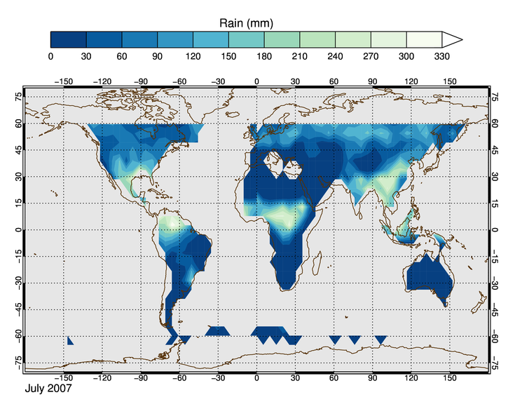 |
| An HDF-EOS gridded field displayed as a filled contour plot. |
![]()
Version of IDL used to prepare this article: IDL 7.1.
![]()
![]()


