
Subsetting an Image with Map Coordinates


QUESTION: I downloaded an image, named IBCAO_V3_500m_SM.tif, from a NOAA web page. The metadata for this image is shown here.
   IBCAO_V3_500m_SM
   Resolution: 500 x 500 m grid cells
   Projection: Polar stereographic, true scale 75degN,
       latitude of origin 90degN, longitude of origin 0deg.
   Horizontal Datum: WGS84
   Vertical Datum: Mean Sea Level
   Extent (Polar stereographic coordinates):
     Easting -2904000 to 2904000;
     Northing -2904000 to 2904000
   Grid dimension: 11617 x 11617
I am interested in a portion of this image from 80 degrees west to 30 degrees west in longitude, and from 64 degrees north to 78 degress north in latitude. Can you show me how to extract this portion of the image for my study?
![]()
ANSWER: The first step is to read the image and reverse it in the Y dimension. This is always necessary for TIFF images that are in map projection space, which always assumes the origin of the map is in the upper left corner of the image, not the lower left corner that IDL assumes.
   file = 'IBCAO_V3_500m_SM.tif'
   image = Read_Tiff(file)
   image = Reverse(image, 2)
The next step is to set up a map coordinate object that describes the image. The information required to do so comes directly from the metadata.
   mapCoord = Obj_New('cgMap', 'Polar Stereographic', Ellipsoid='WGS 84', $
      Center_Longitude=0, True_Scale_Latitude=75, $
      XRange=[-2904000.d, 2904000.d], YRange=[-2904000.d, 2904000.d])
A quick look the histogram plot of the data with the cgHistoplot command shows that the vast majority of values in the image fall between -4000 and 4000. We will use these values to scale the data for display. We load a color table and display the image, with map annotations, with these commands.
   cgLoadCT, 4, /Brewer, /Reverse
   cgDisplay, 1000, 1000, Aspect=image
   cgImage, image, /Keep_Aspect, OPosition=opos, /Save, /Scale, $
       MinValue=-4000, MaxValue=4000
   mapCoord -> SetProperty, Position=opos
   cgMap_Continents, Map=mapCoord
   cgMap_Grid, Map=mapCoord, /Label, Lats=[Findgen(5)*10+40, 85], $
       Lons=Findgen(19)*20.0, LonLab=75, LatLab = 0, Color='charcoal'
You see the result in the figure below.
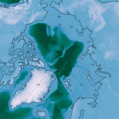 |
| The downloaded image with map annotations added. |
Next, we outline the area of the image you are interested in with with these commands.
   area = mapCoord -> Forward([-80, -80, -30, -30, -80], $
                              [ 78,  64,  64,  78,  78], /NoForwardFix)
   cgPlotS, area, Color='dark red', Thick=2
You see the area, outlined in red below.
 |
| The study area is outlined in red. |
To subset this portion of the image, we need to know the pixel locations associated with the rectangular area that surrounds the study area. The easiest way to do this is to create vectors that describe the XY projected meter space of the image and to look for our region in those vector. The Value_Locate function is perfect for this task. Here is the code. Note that my vectors now describe the outside of the image, and so require one more element than the size of the image in that particular dimension.
   scale = 500.D ; meters
   xmin = -2904000.D - (scale/2.0)
   xmax = 2904000.D + (scale/2.0)
   ymin = -2904000.D - (scale/2.0)
   ymax = 2904000.D + (scale/2.0)
   xvec = cgScaleVector(DIndgen(11617+1), xmin, xmax)
   yvec = cgScaleVector(DIndgen(11617+1), ymin, ymax)
   xpixel = Value_Locate(xvec, [Min(area[0,*]), Max(area[0,*])])
   ypixel = Value_Locate(yvec, [Min(area[1,*]), Max(area[1,*])])
We can draw the rectangular region we are extracting on the image itself, with these commands.
   x0 = Min(area[0,*])
   x1 = Max(area[0,*])
   y0 = Min(area[1,*])
   y1 = Max(area[1,*])
   cgPlots,[x0,x0,x1,x1,x0], [y0,y1,y1,y0,y0], Color='charcoal', SymSize=2, Thick=2
You see the results in the figure below.
 |
| The rectangular area of extraction around the study area. |
The final step is to extract the subimage area and build a map coordinate object that describes the subimage so it can be annotated properly. The code looks like this.
   subImage = image[xpixel[0]:xpixel[1], ypixel[0]:ypixel[1]]
   cgDisplay, WID=1, 500, 500, Aspect=subimage
   cgImage, subimage, /Scale, MinValue=-4000, MaxValue=4000
   subMapCoord = Obj_New('cgMap', 'Polar Stereographic', Ellipsoid='WGS 84', $
      Center_Longitude=0, True_Scale_Latitude=75, Position=[0, 0, 1, 1], $
      XRange=[xvec[xpixel]], YRange=[yvec[ypixel]])
   cgMap_Continents, Map=subMapCoord
   cgMap_Grid, Map=subMapCoord, /Label, Lats=Findgen(12)*2+60, $
      Lons=Findgen(16)*10-180, LonLab=74, LatLab = -140, Color='charcoal'
You see the result in the figure below.
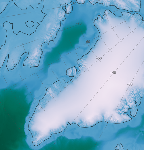 |
| The map annotated subimage extracted from the larger image. |
If you need to, you can produce a mask for your study area. The process is similar to what we have done before. We use PolyFillV to find the indices of the mask pixels. The code looks like this.
   xrange=[xvec[xpixel]]
   yrange=[yvec[ypixel]]
   dims = Size(subimage, /Dimensions)
   xvector = cgScaleVector(DIndgen(dims[0]), xrange[0], xrange[1])
   yvector = cgScaleVector(DIndgen(dims[1]), yrange[0], yrange[1])
   area = subMapCoord -> Forward([-80, -80, -30, -30, -80], $
                                 [ 78,  64,  64,  78,  78], /NoForwardFix)
   mask = BytArr(dims[0], dims[1])
   xpixels = Value_Locate(xvector, area[0,*])
   ypixels = Value_Locate(yvector, area[1,*])
   indices = PolyFillV(xpixels, ypixels, dims[0], dims[1])
   mask[indices] = 1
To display the masked image, we write this code.
   cgDisplay, WID=2, 500, 500, Aspect=subimage
   scaledImage = BytScl(subImage, Min=-4000, Max=4000, Top=254) + 1B
   cgLoadCT, 4, /Brewer, /Reverse, NColors=254, Bottom=1
   TVLCT, cgColor('white', /Triple), 0
   cgImage, scaledImage * mask, XRange=xrange, YRange=yrange
   cgMap_Continents, Map=subMapCoord
   cgMap_Grid, Map=subMapCoord, /Label, Lats=Findgen(12)*2+60, $
       Lons=Findgen(16)*10-180, LonLab=74, LatLab = -140, Color='charcoal'
You see the results in the figure below.
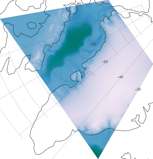 |
| The extracted image masked by the study area. |
A file with the complete code is available.
![]()
Version of IDL used to prepare this article: IDL 8.2.3.
![]()
![]()


