Navigating Map Projected Images

QUESTION: Most of the satellite and remote sensing data I download these days comes in GeoTiff or netCDF files. In the vast majority of cases, the data providers have gridded their data onto map projected meter grids, which are described by metadata in the data files. These image files are easily navigated by creating a map projection space with Map_Proj_Init or the even more useful Coyote Graphics routine, cgMap.

I realize the Map function has not worked properly since it was released in IDL 8.0, but I really was expecting it to be fixed by now in IDL 8.2. But, this appears not to be the case.

What I am trying to do is very simple. I obtain a static map from Google, as a 4x600x600 PNG file, using the code below. This map is centered on Fort Collins, Colorado at latitude 40.6 and longitude -105.1.

   googleStr = "http://maps.googleapis.com/maps/api/staticmap?" + $
      "center=40.6,-105.1&zoom=12&size=600x600" + $
      "&maptype=terrain&sensor=false&format=png32"
   netObject = Obj_New('IDLnetURL')
   void = netObject -> Get(URL=googleStr, FILENAME="googleimg.png")
   Obj_Destroy, netObject
   googleImage = Read_Image('googleimg.png')

I would like to display this image in a graphics window with box axes around it. With Coyote Graphics routines, I use the following code to calculate an X and Y range for the image in projected meter space and to display the image with box axes.

   centerLat = 40.6D
   centerLon = -105.1D
   scale = cgGoogle_MetersPerPixel(12)
   map = Obj_New('cgMap', 'Mercator', ELLIPSOID='WGS 84', /OnImage)
   uv = map -> Forward(centerLon, centerLat)
   uv_xcenter = uv[0,0]
   uv_ycenter = uv[1,0]
   xrange = [uv_xcenter - (300*scale), uv_xcenter + (300*scale)]
   yrange = [uv_ycenter - (300*scale), uv_ycenter + (300*scale)]
   map -> SetProperty, XRANGE=xrange, YRANGE=yrange
   cgDisplay, 700, 700, Title='Google Image with Coyote Graphics'
   cgImage, googleImage, Margin=0.1
   map -> Draw
   cgMap_Grid, MAP=map, /BOX_AXES, /cgGRID
   cgPlotS, -105.1, 40.6, PSYM='filledstar', SYMSIZE=3.0, MAP=map, COLOR='red'

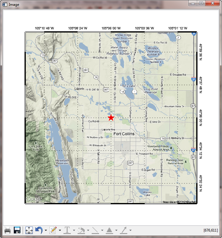
The result of running the code is shown in the figure below. As you can see, the very center of the map is at latitude 40.6 and longitude -105.1.

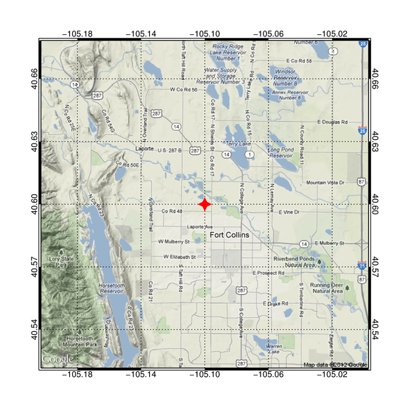A Google static map image displayed with Coyote Graphics routines.

 

Now, I wish to do exactly the same thing using the Map function in IDL 8.2. Can you show me how to do this?

ANSWER: Well, I'll try. No guarantees with Function Graphics routines, though.

A close reading of the documentation (such as it is), leads me to suspect the proper solution will look like this, using the code you have already run.

   obj = Image(googleImage, MAP_PROJECTION='mercator', $ 
         ELLIPSOID='WGS 84', GRID_UNITS=1, $ 
         CENTER_LONGITUDE=centerLon, CENTER_LATITUDE=centerLat, $ 
         XRANGE=xrange, YRANGE=yrange, $
         DIMENSIONS=[700,700], LOCATION=[50,50], /BOX_AXES)

But, running this code results in a completely blank window (although no error message!). When that didn't work, I thought maybe I needed to use the LIMIT keyword, so I tried this.

   ll = map -> Inverse(xrange, yrange)
   limit = [ll[1,0], ll[0,0], ll[1,1], ll[0,1]]
   obj = Image(googleImage, MAP_PROJECTION='mercator', $ 
         ELLIPSOID='WGS 84', GRID_UNITS=1, $ 
         CENTER_LONGITUDE=centerLon, CENTER_LATITUDE=centerLat, $ 
         XRANGE=xrange, YRANGE=yrange, LIMIT=limit, $
         DIMENSIONS=[700,700], LOCATION=[50,50], /BOX_AXES)

That also resulted in a blank window.

Reading much more carefully now, I thought I might try the IMAGE_DIMENSION and IMAGE_LOCATION keywords, and leave the LIMIT keyword off. I tried this.

   xdim = Abs(xrange[1] - xrange[0])
   ydim = Abs(yrange[1] - yrange[0])
   xloc = xrange[0]
   yloc = yrange[0]
   obj = Image(googleImage, MAP_PROJECTION='mercator', $ 
         ELLIPSOID='WGS 84', GRID_UNITS=1, $ 
         CENTER_LONGITUDE=centerLon, CENTER_LATITUDE=centerLat, $ 
         XRANGE=xrange, YRANGE=yrange, $
         DIMENSIONS=[700,700], LOCATION=[50,50], /BOX_AXES, $
         IMAGE_DIMENSIONS=[xdim,ydim], IMAGE_LOCATION=[xloc,yloc])

This resulted in an image displayed! But, it filled up the window instead of having a margin around it. But, as it seemed like I was on the right track, I tried substituting a POSITION keyword for the LOCATION keyword.

   obj = Image(googleImage, MAP_PROJECTION='mercator', $ 
         ELLIPSOID='WGS 84', GRID_UNITS=1, $ 
         CENTER_LONGITUDE=centerLon, CENTER_LATITUDE=centerLat, $ 
         XRANGE=xrange, YRANGE=yrange, $
         DIMENSIONS=[700,700], POSITION=[0.1, 0.1, 0.9, 0.9], /BOX_AXES, $
         IMAGE_DIMENSIONS=[xdim,ydim], IMAGE_LOCATION=[xloc,yloc])

This finally displayed the image properly in the window. And, there was some evidence of a map projection, because I could click in the window and have my location updated in map coordinate space. Unfortunately, the map coordinates were wrong! The center of the image was listed as being at -149.5 in longitude and 40.3 in latitude.

But, maybe this is because the ranges were calculated from a center latitude and longitude of 0.0. I tried this variation in which I left the CENTER_LATITUDE and CENTER_LONGITUDE keywords off the command.

   obj = Image(googleImage, MAP_PROJECTION='mercator', $ 
         ELLIPSOID='WGS 84', GRID_UNITS=1, $ 
         XRANGE=xrange, YRANGE=yrange, $
         DIMENSIONS=[700,700], POSITION=[0.1, 0.1, 0.9, 0.9], /BOX_AXES, $
         IMAGE_DIMENSIONS=[xdim,ydim], IMAGE_LOCATION=[xloc,yloc])

This resulted in something much closer to what I had in mind. I could even put a star on the map at the center of the image. It appeared to be placed in the right location.

   sym = Symbol(centerLon, centerLat, 'star', /DATA, SYM_COLOR='red', $
         SYM_SIZE=3, SYM_FILLED=1)

To clean things up a little bit more, and to make the labeling look like the Coyote Graphics plot, I tried maniuplating the grid like this.

    obj.mapprojection.mapgrid.BOX_AXES = 1 
    obj.mapprojection.mapgrid.BOX_THICK = 10 
    obj.mapprojection.mapgrid.LINESTYLE = 1   
    obj.mapprojection.mapgrid.GRID_LONGITUDE = 0.04   
    obj.mapprojection.mapgrid.GRID_LATITUDE = 0.03   
    obj.mapprojection.mapgrid.LABEL_POSITION = 0 
    obj.mapprojection.mapgrid.LONGITUDE_MIN=-105.18
    obj.mapprojection.mapgrid.LATITUDE_MIN=40.54

You see the final result in the figure below. As you can see, this wasn't too bad, although I still haven't been able to figure out how to get box axes. Maybe that's just asking too darn much from function graphics!

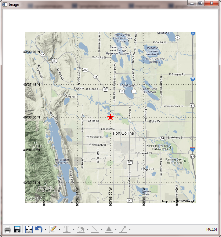A Google static map image displayed with the Map function.

 

You can find a program named mapnogrid.pro that allows you to run the examples shown in this article.

Adding Box Axes

With a little help from the good folks at ExcelisVIS, I finally discovered the correct way to display box axes on my image plot. The secret is to not set the LIMIT and BOX_AXES keywords when you create the image (and, thus, the map projection.) In fact, setting the LIMIT keyword when you create the image is exactly what is causing the graphics window to be blank! This is a known bug in version 8.2 of the software.

Rather, you should set the LIMIT and BOX_AXES properties of the map projection in the interval between when you display the image itself and when you are ready to throw your computer out the second story window!

The correct code to add a box axes looks like this.

   obj = Image(googleImage, MAP_PROJECTION='mercator', $ 
         ELLIPSOID='WGS 84', GRID_UNITS=1, $ 
         XRANGE=xrange, YRANGE=yrange, $
         DIMENSIONS=[700,700], POSITION=[0.05, 0.05, 0.85, 0.85], $
         IMAGE_DIMENSIONS=[xdim,ydim], IMAGE_LOCATION=[xloc,yloc])
    sym = Symbol(centerLon, centerLat, 'star', /DATA, SYM_COLOR='red', SYM_SIZE=3, SYM_FILLED=1)
    obj.mapprojection.mapgrid.LINESTYLE = 1   
    obj.mapprojection.mapgrid.GRID_LONGITUDE = 0.04   
    obj.mapprojection.mapgrid.GRID_LATITUDE = 0.03   
    obj.mapprojection.mapgrid.LABEL_POSITION = 1 
    obj.mapprojection.mapgrid.LONGITUDE_MIN=-105.18
    obj.mapprojection.mapgrid.LATITUDE_MIN=40.54
    obj.mapprojection.mapgrid.BOX_AXES = 1 
    obj.mapprojection.LIMIT = limit  

You see the result in the figure below. The box axes are not labeled like normal box axes, but that is left as an exercise for the reader. Note, too, that setting the limit like this has the effect of blurring the map image just a bit. I think this is probably because the image is now being warped into the map projection, rather than the map projection being applied to the image. You can see the blurring readily, if you compare this image to the one created with Coyote Graphics routines above.

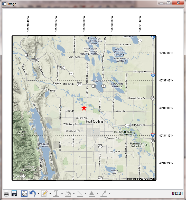A Google static map image displayed with box axes. Note the slight, but noticeable, blurring of the image.

 

Box Axis Labels

An astute reader has written in to say that you can manipulate the map projection labels in the last figure to have a box axis type orientation, by doing something like this.

    lons = obj.mapprojection.mapgrid.LONGITUDES
    FOR j=0,N_ELEMENTS(lons)-1 DO BEGIN
        lons[j].label_angle = 0
        lons[j].label_position = 1
    ENDFOR
    
    ; Then, do the same thing for the latitudes.
    lats = obj.mapprojection.mapgrid.LATITUDES
    FOR j=0,N_ELEMENTS(lats)-1 DO BEGIN
        lats[j].label_angle = 270
        lats[j].label_position = 1
    ENDFOR

You see the result in the figure below. Note that only two sides of the plot can be labeled by this method. If you wanted a normal looking map with box axes, you would have to create your own text labels, presumably.

At least two sides of a map with box axes are labeled using this rotate and position method.

 

Avoid Image Blurring

The image blurring problem described above can be corrected by separating the image display from the creation of the map projection. What is essential to know about this, however, is that the LIMIT keyword to the Map function is broken. (It almost works, but not really. If you try to use the LIMIT keyword, you will get erroneous results.) You must set the limit of the map projection after you create the map object.

The following code will result in an unblurred image with box axes (labeled on only two sides, of course).

   imgObj = Image(googleImage, POSITION=[0.1, 0.1, 0.9, 0.9], DIMENSIONS=[700,700])
   mp = Map('mercator', ELLIPSOID='WGS 84', CENTER_LONGITUDE=centerLon, $ 
         LIMIT=limit, /BOX_AXES, POSITION=[0.1, 0.1, 0.9, 0.9], /CURRENT, $
         GRID_LONGITUDE=0.04, GRID_LATITUDE=0.03, LABEL_POSITION=1, $
         LONGITUDE_MIN=-105.18, LATITUDE_MIN=40.54, LINESTYLE=1, $
         TRUE_SCALE_LATITUDE=0.0)
    sym = Symbol(centerLon, centerLat, 'star', /DATA, SYM_COLOR='red', SYM_SIZE=3, SYM_FILLED=1)
    mp.LIMIT=limit ; MUST do this because LIMIT keyword is broken.
    lons = mp.mapgrid.LONGITUDES
    FOR j=0,N_ELEMENTS(lons)-1 DO BEGIN
        lons[j].label_angle = 0
        lons[j].label_position = 1
    ENDFOR
    lats = mp.mapgrid.LATITUDES
    FOR j=0,N_ELEMENTS(lats)-1 DO BEGIN
        lats[j].label_angle = 270
        lats[j].label_position = 1
    ENDFOR

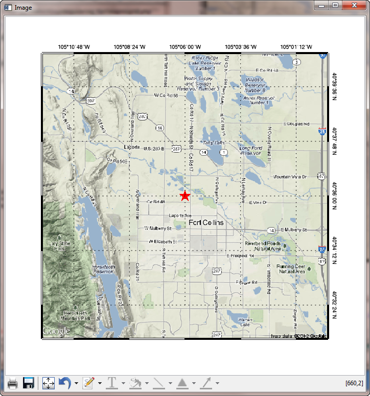
You see the result in the figure below.

A Google static map image displayed with box axes. The image blur has been corrected in this result.

 

Version of IDL used to prepare this article: IDL 8.2.