Displaying an IDL Image in Google Earth

QUESTION: I have a georegistered image with my data that I would like to display in Google Earth. Is it possible to write a KML file from within IDL that I can open in Google Earth to display this image as a ground overlay?

ANSWER: Yes, it is possible to write a KML file from within IDL. You can see an example of this in the Coyote Plot Gallery.

I have needed this capability myself, so I written a number of programs to make this possible. The KML file needed to display an image overlay in Google Earth is a version of an XML file, which is organized as a hierarchy. So, it makes sense to think of implementing a KML writing capability as a hieractical series of objects. Unforunately, this is a big job, so I have decided to chip away at it piecemeal until I have all the pieces I need in place. I started with the object infrastructure I needed to implement what is known in KML as a GroundOverlay object. Essentially, I can write a KML file that will allow you to load any georegistered image (or any image you know the latitude and longitude boundaries of) as a Google Earth overlay.

It is not essential that you know the details of how a KML file is organized. Nor do you even need to know the details of the objects I have created to implement this organization (the object files start with the prefix "cgKML_"). All you really need is an image and the knowledge of where that image should be placed on the Earth. And, you don't even need to know that much if you just know the location of a GeoTiff file which contains the image you wish to see in Google Earth! What I am telling you, in other words, is that writing a KML file to display your IDL image is easy.

All you really need to do is find the cgImage2KML file in the Coyote Graphics Library.

Let's start with a trivial and completely irrelevant example, just to prove the point that any "image" can be displayed in Google Earth. In this case, "image" is any 2D array or true-color image. We are going to use a medical cat scan image and display it covering the United States. We will "locate" the image on the Google Earth map by specifying what KML calls a "LatLonBox". This is just a four-element array that specifies the north, south, west, and east boundaries of the image in that order. The units used are decimal degrees. The code to write a KML file looks like this.

   image = cgDemoData(5)
   cgImage2KML, image, LatLonBox=[48, 25, -125, -75], CTIndex=3, Filename="ctscan.kml", FlyTo=[-100,36,5000]

The cgImage2KML command writes, in your current directory, two files. A file named ctscan.kml, which is the file you load into Google Earth. And a file named ctscan.png, which is the image file that is created from the input image. If you move the KML file to another location, be sure you move its corresponding image file, too, or Google Earth won't be able to locate it. It will assume the image file is in the same directory as the KML file.

You can see what the image looks like when it is opened from within Google Earth in the figure below. (Click any image to see it in a larger format.)

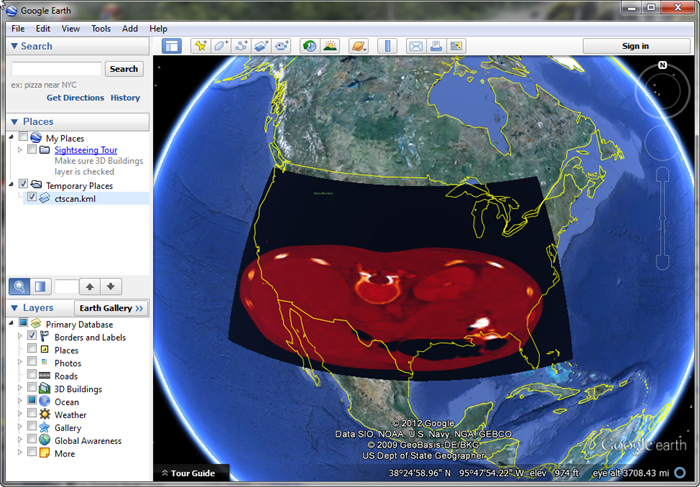An irrelevant medical image displayed in Google Earth to illustrate that any rectangular "image" can be used to create a KML file.

 

We will work with more realistic images in a moment, but before we do, I want to introduce you to two more keywords that will make your image overlays more useful to you. This image has a lot of black pixels. These have a value of 0 in the input image. And we have simply laid this image onto the map. We might want to see some of the terrain underlying the image by making the image transparent. We can set the transparency with the Transparent keyword (to 50% transparent) and we can make all the black pixels totally transparent with the Missing_Value keyword. Here is the code.

   image = cgDemoData(5)
   cgImage2KML, image, LatLonBox=[48, 25, -125, -75], CTIndex=3, Filename="ctscan_transparent.kml", $
        Transparent=50, Missing_Value=0, FlyTo=[-100,36,5000]

You see the results in the figure below.

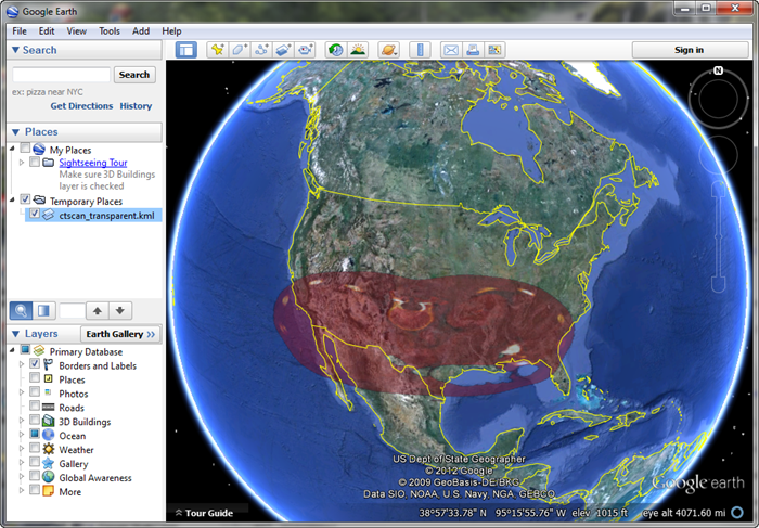This is the same medical image, with transparency turned on in cgImage2KML.

 

Science Images

Let's switch to more relevant, science images. Consider the precipitation data discussed in the article Mapping to a Projected Image. We can download the data file and run the Precipmap program described in the article, to obtain the data, the color palette used to display the data, and the map coordinate object used to describe the map projection and data range used with this data.

   Precipmap, 'ST4.2005010112.24h.bin', DATA=data, PALETTE=palette, MAP=map

Here is the resulting output from running the program.

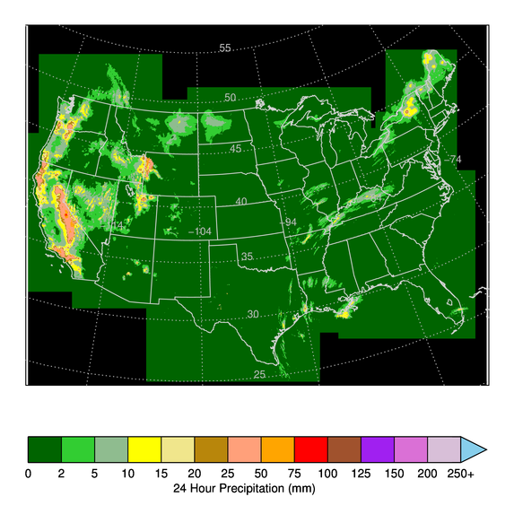Precipitation data in a Polar Stereographic map projection with a spheriod ellipsoid to locate latitude and longitude.

 

This data is in a Stereographic map projection, and it uses a spherical ellipsoid to identify the latitude and longitude points in the map projection, as you can see here.

   IDL> mapInfo = map -> MapInfo()
   IDL> Print, mapInfo.projection, '   ' , mapInfo.datum
        Polar Stereographic   Sphere

This is a problem, because Google Earth requires that the data be in an Equirectangular map projection with a WGS 84 ellipsoid. If you just tried to overlay this data onto Google Earth in its current form, it wouldn't align properly. To overlay this data correctly, you need to warp it from its current map projection into the one supported by Google Earth. The Coyote Library function cgChangeMapProjection does this by using the Map_Proj_Image program. Fortunately, you don't have to worry about this because the call to cgChangeMapProjection is built into the cgImage2KML program. In this case, the missing data is identified by the value of 15. Here is the code to create the KML file. We add a "description" of the data, which appears in the Google Earth interface.

   cgImage2KML, data, map, Palette=palette, Filename="precipitation.kml", $
       Missing_Value=15, Transparent=30, Description='24-Hour Precipition'

You see the result in the figure below.

Precipitation data warped into the Google Earth map projection.

 

GeoTiff Image Files

The situation is even easier of your image files are georegistered and stored in GeooTiff files. The cgImage2KML program can convert such programs to KML files directly. Consider the GeoTiff image containing AVHRR NDVI data discussed in the article Automatically Register GeoTiff Images. The file, AF03sep15b.n16-VIg.tif, can be downloaded here.

Here is the command to create the KML file for this GeoTiff image.

   cgImage2KML, GeoTiff='AF03sep15b.n16-VIg.tif', Min_Value=0, CTIndex=11, $
      /Brewer, /Reverse, Transparent=50, Filename='avhrr_ndvi.kml', $
      Description='AVHRR NDVI Data from Africa', FlyTo=[23,10,11000.]

You see the result in the figure below.

A KML file built directly from a GeoTiff file.

 

Overlapping Images

Google Earth is an excellent tool for comparing how images register or overlap with one another. Here is an example from my own work. I have a classified zonal map, and I want to see where a Landsat scene overlaps the zonal map. The zonal map is in a GeoTiff file with a color palette of only six colors. The Landsat scene is byte scaled from 0 to 127, but this particular scene has extremely low contrast, so I have to scale the image data before I pass it to cgImage2KML, otherwise I don't see the detail in the image that I want to see. To get the Landsat data to overlap the zonal map data, I set the DrawOrder keyword to 1 for the Landsat data. Images with a higher draw order are closer to the viewer's eye in Google Earth. Here is the code I used.

   zoneMap = cgGeoMap('zonal_map.tif', Image=zoneImage, Palette=palette)
   cgImage2KML, zoneImage, zoneMap, Palette=palette, Filename='zonemap.kml', $
       Missing_Value=0, Transparent=50
   landMap = cgGeomap('19730630_241_068_b4.tif', Image=landImage)
   scaledImage = cgImgScl(landImage, MINValue=10, MAXValue=16, /Scale, Missing_Index=0)
   cgImage2KML, scaledImage, landMap, DrawOrder=1, CTIndex=0, Filename='landsat_b4.kml', $
       Missing_Value=0, Transparent=30

You see the results in the figure below.

Images can be made to overlap by setting the draw order with the DrawOrder keyword.

 

These LandSat images are very large (the zone image is 7100 by 6907). I don't need that large an image to view in Google Earth, so I can use the Resize_Factor keyword to reduce (or expand, if needed) the image in size before I create the KML image that will be overlaid. For example, to save time loading the image, I can reduce by image to 25 percent of their original size by setting the Resize_Factor keyword to 0.25.

   zoneMap = cgGeoMap('zonal_map.tif', Image=zoneImage, Palette=palette)
   cgImage2KML, zoneImage, zoneMap, Palette=palette, Filename='zonemap.kml', $
       Missing_Value=0, Transparent=50, Resize_Factor=0.25
   landMap = cgGeomap('19730630_241_068_b4.tif', Image=landImage)
   scaledImage = cgImgScl(landImage, MINValue=10, MAXValue=16, /Scale, Missing_Index=0)
   cgImage2KML, scaledImage, landMap, DrawOrder=1, CTIndex=0, Filename='landsat_b4.kml', $
       Missing_Value=0, Transparent=30, Resize_Factor=0.25

The output is unchanged.

Adding a KML Color Bar

In the last example, we made multiple KML image files that we opened in Google Earth. If you would like to put multiple images (and/or color bars) in the same file, then you have to use the AddToFile keyword available in both cgImage2KML and cgCBar2KML. Here is code that demonstrates how to use the precipitation image we used previously to overlay the precipitation data with a KML color bar added to the display. The cgCBar2KML color bar program can be used to create a stand-alone color bar KML file, or it can added to the same KML file as the image. It takes most of the same keywords as the cgColorbar program.

   kmlFile = Obj_New('cgKML_File', 'precipmap.kml')
   precipmap, 'C:\IDL\ST4.2005010112.24h.bin', DATA=data, PALETTE=palette, MAP=map
   cgImage2KML, data, map, Palette=palette, Missing_Value=15, $
      Description='24-Hour Precipition', PlaceName='Precipitation', $
      FlyTo=[-98,39,11000], AddToFile=kmlFile

   colors = ['dark green', 'lime green', 'light sea green', 'yellow', 'khaki', $
             'dark goldenrod', 'light salmon', 'orange', 'red', 'sienna', 'purple', $
             'orchid', 'thistle', 'sky blue', 'black']
   TVLCT, cgColor(colors, /Triple), 1
   levels = [0, 2, 5, 10, 15, 20, 25, 50, 75, 100, 125, 150, 200, 250]
   cgCBar2KML, NColors=13, Bottom=1, Divisions=14, Title='24 Hour Precipitation (mm)', $
      /Discrete, OOB_High=14, TickNames = StrTrim(levels,2), Charsize=1.5, $
          Description='Precipitation Values', $
          PlaceName='Precipitation Color Bar', $
          AddToFile=kmlFile, Width=400
  kmlFile -> Save
  kmlFile -> Destroy

If you open the precipmap.kml file in Google Earth, you should see something similar to the example below.

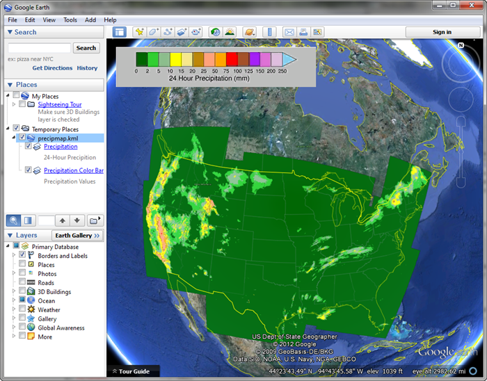KML Color bars can be added to the display."

 

Version of IDL used to prepare this article: IDL 8.2.1.