Mapping to a Projected Image

QUESTION: I have a precipitation image that has already been warped into a polar stereographic map projection. I know the latitude and longitude locations of the four corners of the image, and I know how big the image is. I realize IDL normally warps an image into a map projection space, but I want to do the opposite. I want to warp a map projection space onto the image. Is this possible to do in IDL?

Here is what I know about the image.

   # It is a 1121x881 polar stereographic grid.
   # Point (1,1) is at 23.117N 119.023W.
   # Point (1,881) is at 53.509N 134.039W.
   # Point (1121,1) is at 19.805N 80.750W.
   # Point (1121,881) is at 45.619N 59.959W.
   # The y-axis is parallel to 105W.
   # The resolution is 4.7625km at 60N.
   # The pole point is (I,J) = (400.5,1600.5)

Information about downloading the data and displaying it can be found on this web page. This is a Stage IV data product of 24-hour precipitation accumulation.

ANSWER: The data is distributed in GRIB format, which IDL does not read directly. My thanks to Daniel Vila, who provided the 1121 by 881 data set in an unfomatted binary file. Daniel also alerted me to the fact that missing data in this file was represented by the the value 9.999e20. The demo data set, ST4.2005010112.24h.bin, is available to download.

And special thanks to James Kuyper, who provided the essential algorithm for solving this problem in a 28 April 2006 article he posted on the IDL newsgroup. A more up-to-date version of the program described here can be downloaded from the Coyote Plot Gallery.

To start with, it will be helpful to know what it is we are trying to find. I started by drawing a polar stereographic map projection in a window, and outlining the position of the image on the map. I could do this because I was given the latitude and longitude coordinates of the four corners of the image.

   cgDisplay, 500, 500
   cgMap_Set, /Stereographic, 90, 0, /Continents, /USA, /Grid, /Isotropic, $
       Color='black', /NoErase, /Horizon, Position=[0,0,1,1]
   longitude = [-119.023D, -134.039, -59.959, -80.7500, -119.023]
   latitude = [   23.117D,   53.509,  45.619,  19.8057,   23.117]
   cgPlotS, longitude, latitude, Color='red'
   cgPlotS, -119.023, 23.117, PSym=2, Color='green'

Here is how my map looked after issuing these commands. Essentially what we want to do is rotate that map around and look at it as if through a rectangular window the same size as the image. The green dot on the image shows the lower-left corner of the image.

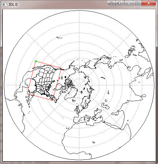A polar stereographic map projection, with outline of the image.

Processing the Image

Before I do that, however, I need to do some processing of the image data. A close look at the NOAA web page indicated the precipitation is normally displayed with a non-linear scaling. This was exciting to me because I had always wondered how to get my cgColorbar program to represent such scaling. A weird map projection wasn't enough of a challenge. This added yet more excitement to my day!

I opened and read the image data file provided by Daniel like this.

   OpenR, lun, 'ST4.2005010112.24h.bin', /Get_Lun
   image = FltArr(1121, 881)
   ReadU, lun, image
   Free_Lun, lun

It didn't occur to me until later that I might have byte-order problems, but I didn't. So presumably that data set came from a little endian machine, like the one I was reading it on. If I was reading this on a big endian machine, I would add a SWAP_IF_BIG_ENDIAN keyword to the OPENR command.

I looked at the NOAA web page again, and saw that they were representing this precipitation data in 14 colors. I set the colors up like this, using a 15th color, black, to represent missing data values. I tried to find colors that were similar to the colors on the NOAA web page. I made substitutions for some of their poorer choices. Notice I avoid loading colors at color index 0 and 255. This is just standard procedure for anything I might want to represent in PostScript.

   colors = ['dark green', 'lime green', 'light sea green', 'yellow', 'khaki', $
             'dark goldenrod', 'light salmon', 'orange', 'red', 'sienna', 'purple', $
             'orchid', 'thistle', 'sky blue', 'black']
   TVLCT, cgColor(colors, /Triple), 1

The levels, as I say, were non-linear. Here are the levels in which precipition was measured.

   levels = [0, 2, 5, 10, 15, 20, 25, 50, 75, 100, 125, 150, 200, 250]

I want to search my image for pixels in those data ranges (which are mm per 24-hour period, by the way). I also want to find the missing pixels. Here is how I did it.

   s = Size(image, /Dimensions)
   scaledImage = BytArr(s[0],s[1])
   FOR j=1,13 DO BEGIN
      index = Where(image GE levels[j-1] AND image LT levels[j], count)
      IF count GT 0 THEN scaledImage[index] = Byte(j)
   ENDFOR
   index = Where(image GT 250 AND image LT 9.999e20, count)
   IF count GT 0 THEN scaledImage[index] = 14B
   missing = Where(image EQ 9.999e20, missing_count)
   IF missing_count GT 0 THEN scaledImage[missing] = 15B

Now my variable, scaledImage, is scaled into the 15 colors (14 data colors and one missing data color) I plan to use to display the image. I am ready to set up my map coordinate space.

Setting up the Map Projection Space

The first step is to set up the map projection space. I know this image is in a Polar Stereographic map projection, and I know from the information you supplied with the image that the center longitude is at 105 degrees west, or -105 in IDL's way of specifying longitude. The CENTER_LATITUTE keyword specifies (oddly!) the latitude of true-scale in a polar map projection. (Even more oddly, the TRUE_SCALE_LATITUDE keyword doesn't work with polar stereographic map projections, although this has been fixed in IDL 8.0.) The latitude of true scale is usually 70 degrees, which is what I will use here. Note that a map structure is returned from the function. This map structure will be used subsequently when we annotate the image.

   mapCoord = Obj_New('cgMap', "Polar Stereographic", $
       CENTER_LONGITUDE=-105, CENTER_LATITUDE=70)

Next, I transform the four corners of my image into UV coordinates. These are just XY Cartesian coordinates associated with a flat 2D space. You could think of it as a box that describes the image. The units are meters, but don't worry about that for now. The U direction is the X direction normally associated with longitude, and the V direction is the Y direction normally associated with latitude. The conversion code looks like this.

   longitude = [-119.023D, -134.039, -59.959, -80.7500]
   latitude =  [  23.117D,   53.509,  45.619,  19.8057]
   uv = mapCoord -> Forward(longitude, latitude)

The latitude and longitude values I just used represent the centers of the corner pixels. But I want to find a box that completely encloses the image. Thus, I need to subtract half a pixel distance from one side of the box and add half a pixel distance to the other side. I can do this in various ways, but I'll start by finding the UV values that are at the top, bottom, and sides of the image box currently. I need these values because I want to calculate the scale of the image in the UV space, as I will need this information shortly.

   topv =   (uv[1,1] + uv[1,2]) * 0.5
   botv =   (uv[1,0] + uv[1,3]) * 0.5
   leftu =  (uv[0,0] + uv[0,1]) * 0.5
   rightu = (uv[0,2] + uv[0,3]) * 0.5

From these values, I can calculate the scaling of each pixel in my UV coordinate space. I need to know this because I have located the top, bottom, and sides of my image in terms of the center of these pixels. (See the original description of the image.) IDL doesn't use pixel centers, it uses pixel edges when it sets up a map coordinate system. Thus, I have to move the values I just found in the code above one half of a pixel towards their respective edges of the image. I find the XY scales associated with this UV coordinate space by dividing the left/right sides, and top/bottom edges by the size of the image. Thus, I know how many units (in UV coordinate space) are associated with a single pixel.

   xscale = (rightu-leftu) / (s[0]-1)
   yscale = (topv-botv) / (s[1]-1)

With the scales I can now calculate the range, in U and V, of the image in UV coordinates. Note that I have to essentially add an extra pixel to the ranges in this step to account for the fact that IDL uses pixel edges for it's map projections, while my image uses pixel centers.

   xrange = [uv[0,1] - (0.5 * xscale), uv[0,2] + (0.5 * xscale)]
   yrange = [uv[1,0] - (0.5 * yscale), uv[1,1] + (0.5 * yscale)]

I will use the UV ranges to set up the mapping coordinate system in such a way that I can draw overlays on the image later in the program.

Displaying the Image Data with the Map

Now it all comes together in a window. Since I like to write programs that don't care what size the window is, or even if the “window” is a PostScript file, I am going to use the POSITION keyword to position the image in the window. This will, by extension, also position the map projection in the window.

Note that I will almost certainly be changing the image size, but want to keep the image aspect ratio by setting the KEEP_ASPECT keyword. Note that the variable pos will contain, when it returns from cgImage, the exact location where the image was placed in the display window.

   cgDisplay, 500, 500
   pos = [0.05, 0.25, 0.95, 0.95]
   cgImage, scaledImage, POSITION=pos, /KEEP_ASPECT

The position variable, pos, may have changed, since I am keeping the image aspect ratio and the position may have had to be adjusted to fit into the window properly. If it has, no problem. I just use this to set up the map projection space, using the UV ranges (which I just calculated) to determine the limits of the projection space. To set up the map projection space, I simply call the Draw method on my map coordinate object.

   mapCoord -> Draw

Now I can draw my continental and USA outlines, as well as grid labels.

   cgMap_Continents, /HIRES, Color='medium gray', /USA, MAP=mapCoord
   cgMap_Grid, LATS=Indgen(8)*5+Round(MIN(latitude)), /LABEL, $
             LONS = Indgen(8)*10+Round(Min(longitude)), $
             COLOR='gray', MAP=mapCoord

And finally, I am ready to put a color bar on my map to indicate the precipitation levels. This is a bit of a problem because the color bar uses a non-linear scale. Essentially what I have to do is trick the color bar into thinking it is using a linear scale, but label the axis with non-linear labels. The only way to do this is to use a tick formatting function, which I have named PrecipMap_Annotate. The call to the cgColorbar program looks like this.

   cgColorbar, NColors=13, Bottom=1, Position=[pos[0], 0.1, pos[2], 0.15], $
      Divisions=14, Title='24 Hour Precipitation (mm)', AnnotateColor='black', $
      /Discrete, OOB_High=14, XTickFormat='PrecipMap_Annotate'

And the PrecipMap_Annotate function is written like this.

   FUNCTION PrecipMap_Annotate, axis, index, value
      plevels = Indgen(15)
      levels = [0, 2, 5, 10, 15, 20, 25, 50, 75, 100, 125, 150, 200, 250]
      labels = StrTrim(levels, 2)
      text = [labels[0:12], labels[13] + '+', '']
      selection = Where(plevels eQ value)
      RETURN, (text[selection])[0]     
   END

You can download my example program, named PrecipMap. The figure below shows you the outcome of running the program.

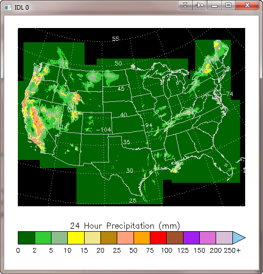A polar stereographic map projection has been placed on an image.

Gridded Data Rather than an Image

Of course, the 2D array you have may not be an image. It could be gridded data that you wish to display on a map projection with the Contour command, for example. If that were the case, you might need to create longitude and latitude vectors to go with your data, since it is not possible to overplot contour data onto a map projection without such vectors. (That is, the Contour command, when used with map projections, will require all three positional parameters be present. You will not be able to pass just a single positional parameter.)

You can easily construct such vectors from the xrange and yrange variables you created above. (cgScaleVector is a Coyote Library program.)

   s = Size(image, /DIMENSIONS)
   lonVector = cgScaleVector(Findgen(s[0]), xrange[0], xrange[1])
   latVector = cgScaleVector(Findgen(s[1]), yrange[0], yrange[1])

Then you could use these vectors to draw a filled contour plot with map boundaries and grids overlaid. Remember to use the keyword CELL_FILL and not FILL when overlaying contours on a map projection, and to calculate the contour levels yourself.

   cgDisplay, 500, 500, WID=1
   colors = ['dark green', 'lime green', 'light sea green', 'yellow', 'khaki', $
             'dark goldenrod', 'light salmon', 'orange', 'red', 'sienna', 'purple', $
             'orchid', 'thistle', 'sky blue', 'black']
   levels = [0, 2, 5, 10, 15, 20, 25, 50, 75, 100, 125, 150, 200, 250]
   TVLCT, cgColor(colors, /Triple), 1
   mapStruct = map_Proj_Init("POLAR STEREOGRAPHIC", $
       CENTER_LONGITUDE=-105, CENTER_LATITUDE=70)
   pos = [0.1, 0.25, 0.9, 0.9]
   cgPlot, xrange, yrange, XSTYLE=5, YSTYLE=21, /NODATA, /NOERASE, POSITION=pos
   cgPlotS, [xrange[0], xrange[0], xrange[1], xrange[1], xrange[0]], $
       [yrange[0], yrange[1], yrange[1], yrange[0], yrange[0]], $
       COLOR='gray'
   missing = Where(image EQ 9.999e20, missing_count)
   IF missing_count GT 0 THEN image[missing] = !Values.F_NAN
   cgContour, image, lonVector, latVector, LEVELS=levels, /CELL_FILL, $
       C_Colors=Indgen(15)+1, /OVERPLOT
   cgMap_Continents, /HIRES, COLOR='light gray', /USA, MAP_STRUCTURE=mapStruct
   cgMap_Grid, LATS=Indgen(8)*5+Round(MIN(latitude)), /LABEL, $
        LONS = Indgen(8)*10+Round(Min(longitude)), $
        COLOR='light gray', MAP_STRUCTURE=mapStruct
   cgColorbar, NColors=13, Bottom=1, Position=[pos[0], 0.1, pos[2], 0.15], $
      Divisions=14, Title='24 Hour Precipitation (mm)', AnnotateColor='black', $
      /Discrete, OOB_High=14, XTickFormat='PrecipMap_Annotate'

You see the result in the figure below.

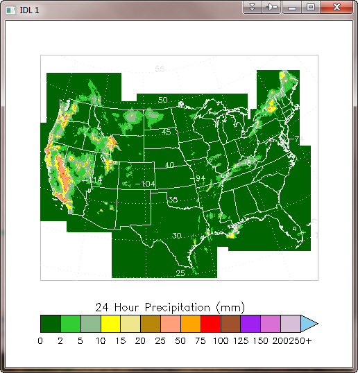The data has been displayed as a filled contour plot on a map projection.