
Annotating GeoTiff Images
QUESTION: I have an AVHRR NDVI image in GeoTIFF format that has been gridded to a particular map projection (an Albers Equal Area projection in this case). I would like to know how to add map annotations such as country outlines and map grid lines to this image. Can you show me how to do this both in Coyote Graphics and in the new Function Graphics?
![]()
ANSWER: The first step in both the Coyote and function graphics system is to read the GeoTiff file and obtain the geotags containing projection information from the file. Once the image is read, you have to reverse it in the Y direction, since all map projection software assumes the (0,0) pixel is in the upper-left corner of the image as you face it. IDL, alone among image processing software, puts that pixel in the lower-left corner by default.
  geoFile = 'AF03sep15b.n16-VIg.tif'
  geoImage= Read_Tiff(geoFile, GeoTIFF=geotag)
  geoImage= Reverse(geoImage, 2)
Next, you use the geotag information to get the pixel scales (number of meters per pixel in the projected image) and the tie point (the location, in projected meter space, of the upper-left corner of the (0,0) pixel). By combining this information with the size of the image in pixels, you can calculate the end points of a coordinate system in projected meter space that completely surrounds the image itself. We will define this data Cartesian coordinate space with the variables xrange and yrange. Note that the origin of the Cartesian coordinate space (the XY axis system) is positioned in the normal way in which more positive X values are to the right and more positive Y values are above any location on the axes.
  xscale  = geotag.ModelPixelScaleTag[0]
  yscale  = geotag.ModelPixelScaleTag[1]
  tp      = geotag.ModelTiePointTag[3:4]
  s = Size(geoImage, /Dimensions)
  xrange = [tp[0], tp[0] + (xscale * s[0])]
  yrange = [tp[1] - (yscale * s[1]), tp[1]]
This image has missing values, indicated by the value -10000.0, so we have to find this value and scale the other values for display.
   missing = Where(geoImage EQ -10000, missingCount)
   IF missingCount GT 0 THEN geoImage[missing] = !Values.F_NaN
   scaled = BytScl(geoImage, Top=254, /NaN)
   IF missingCount GT 0 THEN scaled[missing] = 255
Next, we load the colors for the image display. The "missing" values will be displayed in a white color.
   cgLoadCT, 33, NColors=254
   TVLCT, cgColor('white', /Triple), 255
So far, the code is identical for both the Coyote Graphics program and the Function graphics program. But, now it diverges. We consider the Coyote Graphics example first.
![]()
Coyote Graphics Example
The first thing that is different in the two graphics systems is that the Coyote Graphics map projection routines require that we create a map structure with Map_Proj_Init. This step is incorporated into the Image() function in Function Graphics. We again use information from the geotags to help us set up the map structure. The OnImage keyword tells the cgMap object to gets its position in the output graphics window from the last position used by cgImage.
    alberMap = Obj_New('cgMap', 'Albers Equal Area Conic', $
       DATUM='WGS 84', /ONIMAGE, XRANGE=xrange, YRANGE=yrange, $
       CENTER_LATITUDE=geotag.PROJNATORIGINLATGEOKEY, $
       CENTER_LONGITUDE=geotag.PROJNATORIGINLONGGEOKEY, $
       STANDARD_PAR1=geotag.PROJSTDPARALLEL1GEOKEY, $
       STANDARD_PAR2=geotag.PROJSTDPARALLEL2GEOKEY)
Note that the map projection and datum are hard-coded in this example. But this information is also available in the GeoTiff file. Programs such as cgGeoMap can read this information directly out of the GeoTiff file and create the cgMap object automatically. In other words, a much faster way to create this map object is like this.
alberMap = cgGeoMap(geoFile, /ONIMAGE)
Next, the image is displayed in the graphics window. Because the Keep_Aspect keyword is set, the output position (obtained via the OPosition keyword) may be different from the input position. When we call the Draw method on the cgMap object to set up the map data coordinate system, it will get its position in the window from the output position established by cgImage (because we set the OnImage keyword when we created the cgMap object).
   pos = [0.025, 0.025, 0.975, 0.85]
   cgImage, scaled, POSITION=pos, /KEEP_ASPECT, Background='white'
The next step is to set up a data coordinate space so we can draw annotations on the image. The data coordinate space is set in terms of the projected meter coordinates obtained from the GeoTiff file. We simply set call the Draw method on the cgMap object.
alberMap -> Draw
Finally, we add the continental outlines, map grid lines, and a title.
    cgMap_Continents, Color='Dark Slate Blue', Map_Structure=alberMap, /COUNTRIES, /COASTS
    cgMap_Grid, /LABEL, Color='Slate Blue', Map_Structure=alberMap, $
      GLineStyle=1, Lats=Indgen(8)*10-35, Lons=Indgen(8)*10-15, $
      LatLab=-21, LonLab=-39
    cgText, 0.5, 0.9, /Normal, 'AVHRR NDVI GeoTiff Image', CharThick=2, $
       Alignment=0.5
This entire program is available as CG_GeoTiff_Image. Running the program, we obtain the output shown in the figure below. (The PNG output is obtained from cgWindow.)
   cgWindow, 'cg_geotiff_image', filename, WXSize=600, WYSize=500, $
      WBackground='white', WTitle='AVHRR GeoTiff Image'
   cgControl, Create_PNG='cg_geotiff_image'
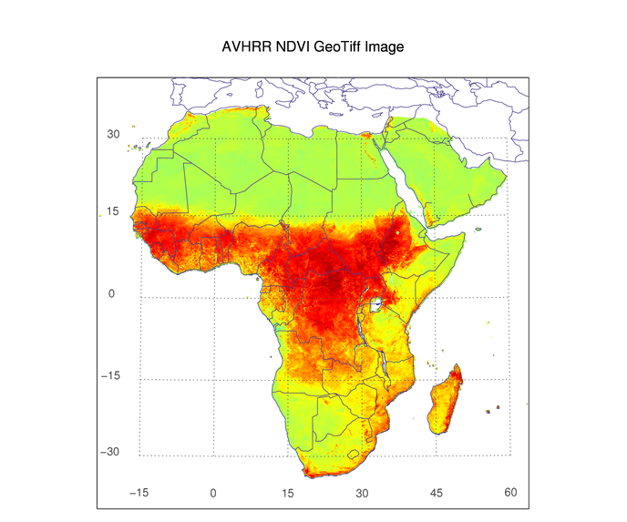 |
| The Coyote Graphics version of annotating a GeoTiff image. |
![]()
Function Graphics Example
In the Function Graphics example, you do exactly the same as before, down to the point where you load the color table for the image. At that point, you have to obtain the color table vectors so you can pass them as a color palette to the image object. Also, you have to calculate the dimensions of the image in the projected XY coordinate system of the GeoTiff file.
   TVLCT, rgb, /Get
   xdim = xrange[1] - xrange[0]
   ydim = yrange[1] - yrange[0]
The next step is to create the Image object, passing it all the map projection information you have collected from the geotags. Do not make the mistake of first creating a map projection object and then adding an image object to that. Along that path lies confusion and broken keywords galore! I don't pretend to understand the Map() function, but it seems extraordinarily hard to control on its own! It is much better behaved from inside an image object. (If you make a map object on its own, the LIMIT, POSITION, XRANGE, and YRANGE keywords all appear to be ignored or broken!)
I know now that my confusion about the map object's keywords is because of a bug in the map object. The bug is scheduled to be fixed in IDL 8.2.
   im = Image(scaled, $
      IMAGE_DIMENSIONS=[xdim,ydim], $
      IMAGE_LOCATION=[xrange[0], yrange[0]], $
      GRID_UNITS='meters', RGB_TABLE=rgb, $
      MAP_PROJECTION='Albers Equal Area', $
      ELLIPSOID='WGS 84', $
      LIMIT=[-35, -30, 40, 60], $
      CENTER_LATITUDE=geotag.PROJNATORIGINLATGEOKEY, $
      CENTER_LONGITUDE=geotag.PROJNATORIGINLONGGEOKEY, $
      STANDARD_PAR1=geotag.PROJSTDPARALLEL1GEOKEY, $
      STANDARD_PAR2=geotag.PROJSTDPARALLEL2GEOKEY, $
      XRANGE=xrange, YRANGE=yrange, $
      POSITION=[0.025, 0.025, 0.975, 0.85])
Next, you can set properties of the map grid. First, obtain the map object from the image object, then obtain the grid object from the map object. Set grid properties as desired.
   map = im.MapProjection
   grid = map.MapGrid
   grid.COLOR = cgColor('charcoal', /Row)
   grid.LINESTYLE = "dotted"
   grid.FONT_SIZE=10
   grid.LABEL_POSITION = 0.05
Finally, add continental outlines and a title for the visualization.
   continents =  MAPCONTINENTS(/COUNTRIES, COLOR=cgColor('charcoal', /Row))
   title = Text(0.5, 0.925, 'AVHRR NDVI GeoTiff Image', $
       FONT_SIZE=14, /NORMAL, ALIGNMENT='center')
This entire program is available as NG_GeoTiff_Image. Running the program, we obtain the output shown in the figure below. (The PNG output is obtained from the graphics window at a resolution of 300 dpi and then reduced by 25% in size for inclusion on the web page.)
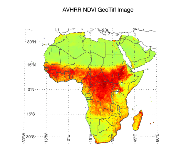 |
| The Function Graphics version of annotating a GeoTiff image. |
![]()
Version of IDL used to prepare this article: IDL 8.1.
![]()
![]()
Updated: 20 November 2011


