
Comparing Filled Contour Plots
QUESTION: I thought it might be interesting to see how the three major graphics systems in IDL deal with placing a filled contour plot on a map projection. I am comparing the venerable Direct Graphics system in IDL, the Coyote Graphics system, and the Function Graphics system that was introduced in IDL 8.0. I am using the latest released version of IDL, which is IDL 8.1, for the comparison.
I have downloaded the original map projected data from the NCEP/DOE Reanalysis II Project. For this comparison, I have chosen a single time step at a single pressure level to contour. I have saved the 2D temperature data array, and the longitude and latitude vectors present in the file, in an IDL save file that you can download from my web page if you would like to perform the experiment yourself.
![]()
ANSWER: The first step is to restore the data file and set up some housekeeping variables that I will use in all three examples. The code to do so looks like this. The saved variables are data, lon, and lat.
  Restore, 'air.nc.data.sav'
  xrange = [Min(lon), Max(lon)]
  yrange = [Min(lat), Max(lat)]
  center_lon = (xrange[1]-xrange[0])/2.0 + xrange[0]
  nlevels = 12
  levels = cgConLevels(Float(data), NLevels=nlevels+1, $
       MinValue=Floor(Min(data)), STEP=step, Factor=1)
  mylat = 40.6  ; Latitude of Fort Collins, Colorado.
  mylon = 254.9 ; Longitude of Fort Collins, Colorado.
  LoadCT, 0
  cgLoadCT, 2, /Reverse, /Brewer, NColors=nlevels-1, Bottom=1
  TVLCT, cgColor('white', /Triple), nlevels
![]()
Direct Graphics Example
The first step here is simply to open a window. The code that follows will use indexed color, as is usual with direct graphics and virtually required if you are going to use the Contour command.
  Window, 2, Title='Direct Graphics Contour Plot'
  Device, Decomposed=0
Next, we set up the map projection space. The data itself is in an equirectangular map projection, but we want to use Map_Set in this example. The closest thing to it is a cylindrical map projection, so we will use that. We will position the map projection so we can display a color bar above it.
  Map_Set, /Cylindrical, 0, 180, Position=[0.1, 0.1, 0.9, 0.8], $
     Limit=[Min(lat), Min(lon), Max(lat), Max(lon)]
The next step is to create the contour plot, and overplot it onto the map projection. We do this in two steps so we can have contour lines separating the filled contour values. We have specified 12 contour intervals in this particular case.
  Contour, data, lon, lat, /Cell_Fill, /Overplot, $
     C_Colors=Indgen(nlevels)+1, Levels=levels
  Contour, data, lon, lat, /Overplot, $
     Color=cgColor('white'), Levels=levels, C_Labels=Replicate(1, 12)
Finally, we add the plot annotations. These include grid lines, continental outlines, a location for Fort Collins, Colorado (added with PlotS) and a color bar. When we are finished we return the device to the default decomposed color state.
  Map_Grid, Color=cgColor('charcoal')
  Map_Grid, /Box, /No_Grid, Color=cgColor('white')
  Map_Continents, Color=cgColor('tomato')
  PlotS, mylon, mylat, PSYM=2, SymSize=2, Color=cgColor('tg1')
  cgColorbar, Range=[Min(levels), Max(levels)-step], OOB_High=nlevels, $
     NColors=nlevels-1, Bottom=1, /Discrete, Color='opposite', $
     Title='Temperature ' + cgSymbol('deg') + 'K', $
     Position=[0.1, 0.91, 0.9, 0.95]
  Device, Decomposed =1
You see the results in the figure below.
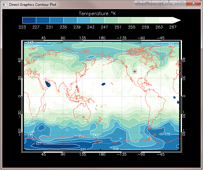 |
| A Direct Graphics filled contour plot with 12 contour levels. Time to render, 0.457 seconds. |
![]()
Coyote Graphics Example
The Coyote Graphics example is similar to the Direct Graphics example, as you would expect. We will, however, display this contour plot in a resizeable graphics window from which you can save the contour plot as a PostScript, PDF, or raster file. The first step is to create the window. We turn command execution off until we are finished entering multiple commands.
  cgWindow, WTitle='Coyote Graphics Contour Plot'
  cgControl, Execute=0
The next step is to set up the map projection space. I want to use the GCTP map projections set up with Map_Proj_Init, but there are many problems in doing so. As if ephemerial map structures weren't enough of a headache, Map_Grid has numerous problems with Map_Proj_Init map spaces that make it extremely frustrating to get labels and grids on the map. Most of these problems (all that I know about, anyway) have been corrected in the Coyote Graphics Map Projection Routines, so I will use these in the code here. It is possible, although much more difficult, to use the Map_Proj_* routines directly.
We set up and establish the map projection space with these commands.
  map = Obj_New('cgMap', 'Equirectangular', Ellipsoid=19, $
     XRange=xrange, YRange=yrange, /LatLon_Ranges, CENTER_LON=center_lon, $
     Position=[0.1, 0.1, 0.9, 0.8], Limit=[Min(lat), Min(lon), Max(lat), Max(lon)])
  map -> AddCmd, Method='Erase'
  map -> AddCmd, Method='Draw'
Next, we draw the contour plot. Notice here we can put the contour outlines on (with the Outline keword) in the same command we use to produce the filled contours.
  cgContour, data, lon, lat, /Cell_Fill, /Overplot, /Outline, $
     C_Colors=Indgen(nlevels)+1, Levels=levels, Map=map, OutColor='White', /AddCmd
Finally, we add the same map annotations we added previously, and allow the commands to execute in the resizeable graphics window.
  cgMap_Grid, Map=map, /Box, /AddCmd
  cgMap_Continents, Map=map, Color='tomato', /AddCmd
  cgColorbar, Range=[Min(levels), Max(levels)-step], OOB_High=nlevels, $
     NColors=nlevels-1, Bottom=1, /Discrete, $
     Title='Temperature ' + cgSymbol('deg') + 'K', $
     Position=[0.1, 0.91, 0.9, 0.95], /AddCmd
  cgPlots, mylon, mylat, PSYM=16, SymSize=2, color='tg1', Map_Object=map, /AddCmd
  cgControl, Execute=1
You see the result in the figure below.
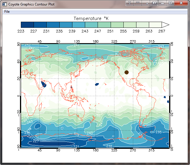 |
| A Coyote Graphics filled contour plot with 12 contour levels in
a resizeable graphics window. Time to render, 0.535 seconds. |
You see a couple of differences with the Direct Graphics result. The contour plot fills to the edges of the map better. And the default labeling is maybe a bit more sensible. But it is similar to the Direct Graphics result. The Coyote Graphics plot is similar to the Function Graphics plot shown below, in that both can automatically produce PostScript, PDF, and high quality raster file output.
![]()
Function Graphics Example
I am using the Contour and Colorbar functions as they are in IDL 8.1 in this example. One can only hope they improve in the next version of IDL. Nevertheless, I am not absolutely sure I have found the most efficient way to write this code. If you have a better idea, I am happy to hear it and I'll update the page immediately. What I am attempting to do here is create the same plot in Function Graphics that we just created in Direct and Coyote Graphics. I have written elsewhere about the myriad problems with the Contour function, so I'll not dwell on those problems here.
The first step is to reload the colors. We have to do this because the Colorbar function cannot deal with less than 256 colors. Here we get the colors we loaded so we can pass them to the Contour function.
   cgLoadCT, 2, /Brewer, /Reverse
   TVLCT, rgb, /Get
Next, we set up the window and turn off updating until we are finished loading the window and manipulating the graphics elements.
   win = Window(Dimension=[640, 512])
   win.Refresh, /Disable
I tried to put a title in the window bar by using the Title keyword to the Window function above, but that put the title in the window where it was overwritten by the color bar. I don't know how to put a title in the actual window bar. If you do, please let me know.
To draw lines on a filled contour plot, it is necessary to create the contour lines first. Otherwise, the labeling on the contour lines is very, very large. We create the contour lines like this. Notice that I have to essentially replicate the filled contour plot in almost every detail. If I don't do this, the two contour plots do not line up correctly.
   overplot = Contour(data, lon, lat, C_Color='gray', $
       C_Label_Show=Replicate(1, 12), C_Use_Label_Orientation=1, $
       Grid_Units=2, Map_Projection='Equirectangular', Font_Size=8, $
       Position=[0.05,0.05,0.95,0.80], RGB_Table=rgb, /Current, $
       C_Label_Interval=0.8, C_VALUE=levels)
Next, I want to hide the map projection properties of this overplot, or they will interfere with the map projection properties of the filled contour plot.
   map = overplot.MapProjection
   map.center_longitude = 180.0
   grid = map.MapGrid
   grid.hide = 1
Now, I create the filled contour plot, and move the contour lines in front. Note that I have used the same Position keyword I used for the two previous plots, but that neither of these contour plots honor the position in the window. They seem to have a mind of their own. If you know how to get them positioned correctly, please contact me.
   dataObj = Contour(data, lon, lat, /Fill, $
       Grid_Units=2, Map_Projection='Equirectangular', $
       Position=[0.05,0.05,0.95,0.80], RGB_Table=rgb, /Current, $
       C_VALUE=levels, RGB_INDICES=BytScl(Indgen(nlevels)))
    overplot.order, /Bring_Forward
Next, I manipulate the map projection properties to try to duplicate the map projection properties of the previous two plots.
   grid = map.MapGrid
   grid.color = cgColor('charcoal', /Triple, /Row)
   grid.linestyle = 1
   grid.grid_longitude = 60
   grid.grid_latitude = 30
   grid.label_position = 0.0
   grid.box_axes = 1
   c = MapContinents(Color=cgColor('tomato', /Triple, /Row), /Current)
Finally, I add a color bar and refresh the window so we can see the results. The color bar requires a fake data object to attach to or it is impossible to get the colors right.
   fakeObj = Contour(cgScaleVector(data, Min(levels), Max(levels)), lon, lat, /Fill, $
       Grid_Units=2, Map_Projection='Equirectangular', $
       Position=[0.05,0.05,0.95,0.80], RGB_Table=rgb, /Current, $
       C_VALUE=levels, Hide=1)
   cb = Colorbar(Target=fakeObj, Tickname=levels[0:nlevels], $
      Major=13, /Border_On, Title='Temperature $\deg$ K', $
      Position=[0.1, 0.88, 0.9, 0.93], Minor=0)
   s = Symbol(mylon, mylat, /Data, /Current, 'Star', /Sym_Filled, Sym_Color='red')
   win.Refresh
You see the results in the figure below. Note that the symbol doesn't show up on the plot. I would like to know how to fix that. If you would like to run this program yourself, you can download an example program. You will need other Coyote Library programs to run the code.
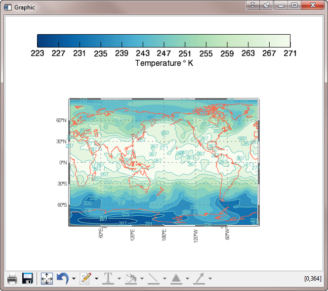 |
| A Function Graphics filled contour plot with 12 contour levels in
a resizeable graphics window. Time to render, 6.028 seconds. |
![]()
IDL 8.2.1 Update
There are reports that function graphics speed has been improved in recent IDL updates. Plus, the Colorbar function has been completely revamped and supposedly works correctly now. To test these claims, I set out to rewrite the Function Graphics code for this purpose. It took a collaborative effort, and many hours over several days to accomplish, but we eventually were able to write a program that duplicated the Coyote Graphics plot.
We had to work around several bugs that are still present in the function graphics system. First of all, we have to use a LIMIT keyword on our map projection command, and make sure the latitude limits did not go all the way from -90 to 90 degrees. If we failed to do this, there were two extra labels on the map projection in erroneous places that we could not get rid of.
  mp = Map('Equirectangular', CENTER_LONGITUDE=180, $
    POSITION=[0.1,0.1,0.90,0.80], $
    LABEL_POSITION = 0, BOX_AXES=1, $
    GRID_LATITUDE = 30, GRID_LONGITUDE = 45, $
    /CURRENT, ASPECT_RATIO=0, LIMIT=[-89.99, 0, 89.99, 360])
Then, we had to create another grid object to label the top and right axes. That code to produce box axes looks like this.
  mp1 = Map('Equirectangular', CENTER_LONGITUDE=180, $
    POSITION=[0.1,0.1,0.90,0.80], $
    LABEL_POSITION = 0, BOX_AXES=1, $
    GRID_LATITUDE = 30, GRID_LONGITUDE = 45, $
    /CURRENT, ASPECT_RATIO=0, LIMIT=[-89.99, 0, 89.99, 360])
  mp1['Latitudes'].label_angle=90
  mp1['Longitudes'].label_angle=0
  grid = MapGrid( $
       LONGITUDE_MIN=0, LONGITUDE_MAX=360, $
       LATITUDE_MIN=-90, LATITUDE_MAX=90, $
       GRID_LONGITUDE=45, GRID_LATITUDE=30, $
       LABEL_POSITION=1)
   FOREACH g,grid.latitudes DO g.label_angle=270
   FOREACH g,grid.longitudes DO g.label_angle=0
But, that said, the graphics rendering time is vastly improved, as you can see in the table at the bottom of the page. It is clear things are moving in the right direction, even if we are not fully there yet.
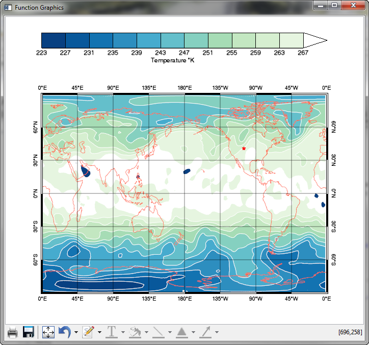 |
| A Function Graphics filled contour plot with 12 contour levels in
a resizeable graphics window. Time to render, 2.9 seconds in IDL 8.2.1. |
![]()
Rendering Speeds of Output
I've been asked to add rendering speeds to this comparison. I've come up with two numbers for each. The first number is for a fresh IDL session. The second is for an experienced IDL session, in which I have already run the program and compiled all the needed procedures and functions. The numbers should be used in a relative sense. I ran the tests on my Windows 7, 64-bit computer, and I timed just the rendering portion of the code (put up a window and display the plot in it).
| Rendered In | Fresh IDL Session | Old IDL Session |
| Direct Graphics | 0.494 | 0.457 |
| Coyote Graphics | 0.727 | 0.535 |
| Function Graphics IDL 8.1.0 | 8.520 | 6.028 |
| Function Graphics IDL 8.2.1 | 4.82 | 2.902 |
| Function Graphics IDL 8.2.3 | 4.800 | 2.124 |
![]()
Version of IDL used to prepare this article: IDL 8.1 and IDL 8.2.1.
![]()
![]()
Updated 2 December 2012


