Device Independent Contour Plots

QUESTION: I realize the Contour command is older than dirt, but it's still pretty useful. Isn't there a way to bring it into the 21st century and make it work with modern computers? I don't want it to do everything. I just want it to solve all my contouring problems. I know you built cgImage, which made the TV command useful again. Couldn't you do something similar for the Contour command?

ANSWER: Humm. Maybe I could.

Here is a list of the features I think such a program should have.

• It should work the same on the display, in a PostScript file, and in the Z-Graphics buffer.
• It should work the same whether you are using decomposed color or indexed color.
• It should use all the same keywords the Contour command uses.
• The NLevels keyword should produce N equally spaced contour levels..
• It should be able to produced filled contour plots.
• It should eliminate the hole that often occurs in contour plots.
• It should have an easy way to select which contours to label.
• It should work with colors intelligently.
• It should be able to overplot contours on images.
• It should handle irregular data.
• It should be capable of being displayed in a resizable graphics window.
• It should allow automatic output to PostScript, PDF, and raster files.

The program I've written is a Coyote Library program named cgContour. It has all of the features listed above. It won't matter if you run the program with decomposed color turned on (what I always recommend!) or if you run the program in indexed color mode. It will work the same on your machine, in a PostScript file, and in the Z-graphics buffer.

Here are some side-by-side comparisons with the original Contour command. Here is the data we are going to work with.

   IDL> data = cgDemoData(2)
   IDL> Help, data
    DATA     FLOAT = Array[41, 41]

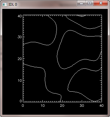
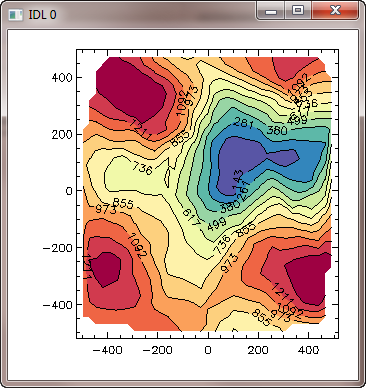
First, the most basic of the contour commands, with only default values.

   IDL> Contour, data
   IDL> cgContour, data

The result of the first command is on the left, and the second command is on the right.

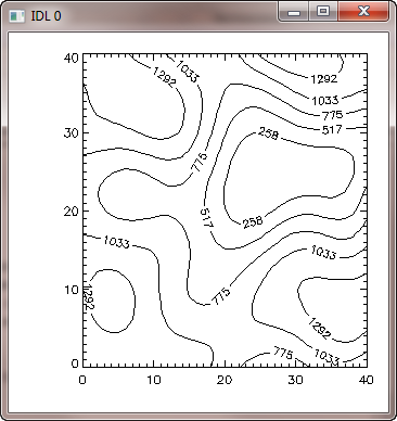The most basic Contour command on the left. The most basic cgContour command on the right.

 

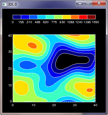
Here is code to compare a simple filled contour plot.

   data = cgDemoData(2)
   cgLoadCT, 33, NColors=10, Bottom=1
   c_colors = Indgen(10)+1
   position = [0.1, 0.1, 0.9, 0.75]

   Contour, data, NLevels=10, /Fill, Position=position, C_Colors=c_colors
   Contour, data, NLevels=10, /Overplot
   cgColorbar, Divisions=10, Range=[Min(data), Max(data)], /Discrete, $
      Position=[0.1, 0.90, 0.9, 0.94], NColors=10, Bottom=1

   cgContour, data, NLevels=10, /Fill, Position=position, C_Colors=c_colors, /Outline
   cgColorbar, Divisions=10, Range=[Min(data), Max(data)], /Discrete, $
      Position=[0.1, 0.90, 0.9, 0.94], NColors=10, Bottom=1

The traditional contour plot is shown on the left, and the Coyote Graphic contour plot result is shown on the right in the figure below.

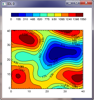A basic filled Contour command on the left. A basic filled cgContour command on the right.

 

Other Features of cgContour

Here are a few of the other features of cgContour.

Easy Labeling of Contour Levels

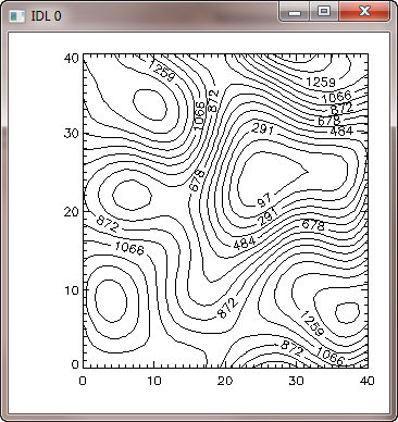
The Label keyword allows you to easily label every contour level (Label=1), every other contour level (Label=2), every third contour level (Label=3), etc. Set Label to 0 to supress contour labelling.

   cgContour, data, NLevels=16, Label=2

Easy labeling of contour levels.

 

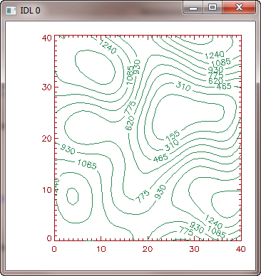
Intelligent Use of Color

Any named color supported by cgColor is allowed for axes and contour data.

   cgContour, data, NLevels=10, AXISCOLOR='red7', COLOR='sea green'

Intelligent use of colors.

 

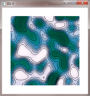
Contours Plotted on Images

Contours can easily be plotted on top of images displayed with cgImage and the OnImage keyword.

   image = cgDemoData(18)
   cgLoadCT, 4, /Brewer, /Reverse
   cgImage, image, Position=[0.1, 0.1, 0.9, 0.9], /Keep_Aspect, /Save
   cgContour, image, NLevels=9, Label=0, /OnImage

Easy overplotting of contours on images.

 

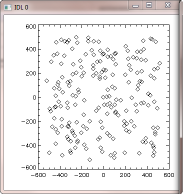
Allow Contouring of Irregular Data

First create some irregular, random data.

   data2d = cgDemoData(2)
   s = Size(data2D, /Dimensions)
   lon = (Indgen(s[0]) * 25000L - 500000L) / 10^3
   lat = (Indgen(s[1]) * 25000L - 500000L) / 10^3
   lat2d = Rebin(Reform(lat, 1, 41), 41, 41)
   lon2d = Rebin(lon, 41, 41)
   pts = Round(RandomU(-3L, 200) * 41 * 41) 
   dataIrr = data2d[pts] 
   lonIrr = lon2d[pts] + RandomU(5L, 200) * 50 - 25
   latIrr = lat2d[pts] + RandomU(8L, 200) * 50 - 25
   LoadCT, 0
   cgPlot, lonIrr, latIrr, PSYM=4

   cgLoadCT, 25, /Brewer, /Reverse
   cgContour, dataIrr, lonIrr, latIrr, NLevels=12, /Irregular, /Fill, /Outline

On the left, locations of randomly sampled points in the data. On the right, a contour plot of the irregular data.

 

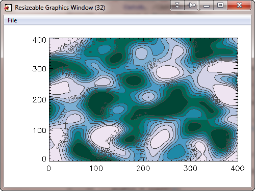
Display in Resizable Graphics Window

To display the command in a resizable graphics window, simply set the Window keyword. Here is a filled contour with outlines, all on the same command.

   image = cgDemoData(18)
   cgLoadCT, 4, /Brewer, /Reverse
   cgContour, image, NLevels=9, /Fill, /Outline, /Window

The contour plot can be displayed in a resizable graphics window.

 

Automatic Output to PostScript, PDF, and Raster Files

The cgContour command, like all Coyote Graphics commands, can automatically create PostScript, PDF, and raster file (BMP, GIF, JPEG, PNG, and TIFF) output. Simply set the Output keyword to the name of the file you want to create.

    data = cgDemoData(2)
    cgLoadCT, 33
    cgContour, data, /Fill, /Outline, Output='myplot.ps'
    cgContour, data, /Fill, /Outline, Output='myplot.pdf'
    cgContour, data, /Fill, /Outline, Output='myplot.png'

Version of IDL used to prepare this article: IDL 7.0.1.